What is Linear Regression In ML? With Example Codes

What is Linear Regression in Machine Learning?

The field of Machine Learning is full of numerous algorithms that allow Data Scientists to perform multiple tasks. To understand an algorithm, it’s important to understand where it lies in the ocean of algorithms present at the moment. There are numerous ways in which all such algorithms can be grouped and divided. Some of these groups include-

Statistical vs. Non-statistical Algorithms

The differentiation between non-statistical and statistical based algorithms is that statistical algorithms use concepts of statistics to solve the common business problem found in the field of Data Science. In contrast, non-statistical algorithms can use a range of methods, which include tree-based, distance-based, probabilistic algorithms.

Business Problems

The other way of defining algorithms is what objective they achieve, and different algorithms solve different business problems. The common business problems include

• Regression Problem:  This is a business problem where we supposed to predict a continuous numerical value
• Classification Problem: Here, we predict a predetermined number of categories
• Segmentation: Also known as clustering, this business problem involves the detection of underlying  patterns in the data so that an apt amount of groups can be formed from the data
• Forecasting: In business forecasting, we predict a value over a period of time. It is different from Regression as there is a time component involved; however, there are situations where regression and forecasting methodologies are used together.

Related: Different Types of Machine Learning Algorithms

Linear and Non-Linear Algorithms

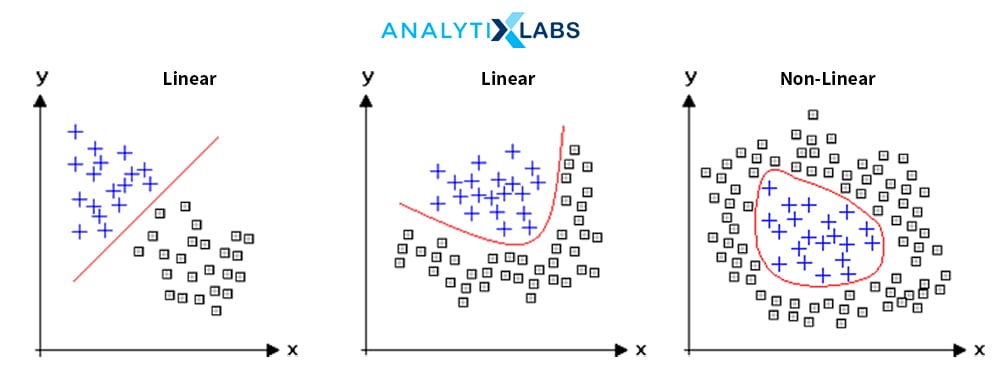
Some algorithms come up with linear predictions, or their decision boundary is linear. In contrast, some algorithms, such as numerous tree-based and distance-based algorithms, come up with a non-linear result with its own advantages (of solving non-linear complicated problems) and disadvantages (of the model becoming too complex).

Interpretability

Some algorithms have the concept of weights or coefficients through which the important predictors can be determined, whereas some algorithms do not have this advantage.

With the above understanding of the numerous types of algorithms, it is now the right time to introduce the most important and common algorithm, which in most cases, is the algorithm that a Data Scientist first learns about – Linear Regression. Given the above definitions, Linear Regression is a statistical and linear algorithm that solves the Regression problem and enjoys a high level of interpretability.

To understand the Linear Regression algorithm, we first need to understand the concept of regression, which belongs to the world of statistics. Regression is a statistical concept that involves establishing a relationship between a predictor (aka independent variables / X variable) and an outcome variable (aka dependent variable / Y variable). These concepts trace their origin to statistical modeling, which uses statistics to come up with predictive models. The Linear Regression concept includes establishing a linear relationship between the Y and one or multiple X variables.

Today, we live in the age of Machine Learning, where mostly complicated mathematical or tree-based algorithms are used to come up with highly accurate predictions. However, even among many complicated algorithms, Linear Regression is one of those “classic” traditional algorithms that have been adapted in Machine learning, and the use of Linear Regression in Machine Learning is profound. As linear regression comes up with a linear relationship, to establish this relationship, a few unknowns such as beta, also known as coefficients, and intercept value, also known as the constant, are to be found. These values can be found using the simple statistical formula as the concepts in themselves are statistical. However, when we use statistical algorithms like Linear Regression in a Machine Learning setup, the unknowns are different.

Under the Machine Learning setup, every business problem goes through the following phases-

1. Identification of the type of problem, i.e., if the problem is a Regression, Classification, Segmentation, or a Forecasting problem.
2. Data preprocessing to have clean and usable data.
3. Selecting the algorithm to solve the problem
4. Coming up with a mathematical equation to establish a relationship between the X and the Y variable (or to perform some other task)
5. Identifying the unknown in the mathematical equation
6. Converting the problem into an optimization problem where a loss function is identified based on which unknowns are found.
7. Using the final known values to solve the business problem

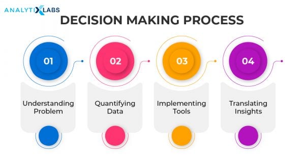
When a statistical algorithm such as Linear regression gets involved in this setup, then here, we use optimization algorithms and the result rather than calculating the unknown using statistical formulas. Thus, this uses linear regression in machine learning rather than a unique concept. It uses the sophisticated methodology of machine learning while keeping the interpretability aspect of a statistical algorithm intact.

What Are The Types of Regression?

As mentioned earlier, regression is a statistical concept of establishing a relationship between the dependency and the independent variables. However, depending upon how this relationship is established, we can develop various types of regressions, with each have their own characteristics, advantages, and disadvantages. Some of the common types of regression are as follows.

1. Linear (OLS) Regression

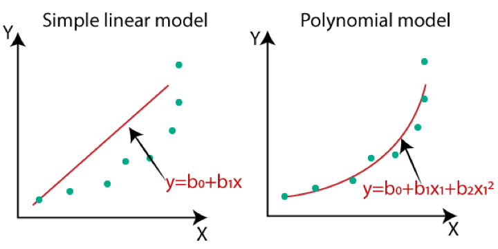
This is the traditional form of regression, where the dependent variable is continuous. To predict this variable, a linear relationship is established between it and the independent variables. Here we come up with a straight line that passes through most data points, and this line acts as the prediction. As the formula for a straight line is Y = mx+c, we have two unknowns, m, and c, and we pick those values of m and c, which provides us with the minimum error. The line providing the minimum error is known as the line of best fit. The definition of error, however, can vary depending upon the accuracy metric. In linear regression, when the error is calculated using the sum of squared error, this type of regression is known as OLS, i.e., Ordinary Least Squared Error Regression. We can have similar kinds of errors, such as MAD Regression, which uses mean absolute deviation to calculate the line of best fit.

2. Polynomial Regression

As Linear Regression is a linear algorithm, it has the limitation of not solving non-linear problems, which is where polynomial regression comes in handy. Unlike linear regression, where the line of best fit is a straight line, we develop a curved line that can deal with non-linear problems. Here we increase the weight of some of the independent variables by increasing their power from 1 to some other higher number.

3. Quantile Regression

Quantile Regression is a unique kind of regression. It addresses the common problems the linear regression algorithm faces, which are susceptible to outliers; distribution is skewed and suffering from heteroscedasticity. We establish the relationship between the independent variables and the dependent variable’s percentiles under this form of regression.

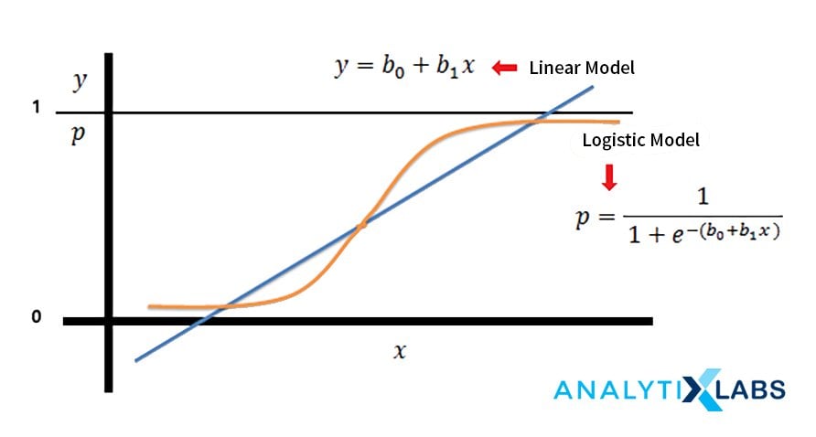
4. Logistic Regression

Part of the Generalized Linear Models, Logistic Regression predicts a categorical dependent variable. Here, a link function, namely logit, is used to develop the predicted probabilities for the dependent variable’s class. Theoretically, the dependent variable should be binary, i.e., only having two categories.

Related: Logistic Regression in R (With Examples)

5. Stepwise Regression

Regression suffers from two major problems- multicollinearity and the curse of dimensionality. To address both these problems, we use Stepwise Regression, where it runs multiple regression by taking a different combination of features. These combinations are created by adding or dropping the variables continuously until the set of features is identified that provides us with the best result.

6. Principal Component Regression

As mentioned above, stepwise addresses the problem of multicollinearity and the curse of dimensionality. This is exactly what this form of regression also does, however, in a very different way. Principal component regression, rather than considering the original set of features, consider the “artificial features,” also known as the principal components, to make predictions. These principle components hold maximum information from the data while at the same time reducing the dimensionality of it. While this method provides us with the advantage of no principal component being correlated and reducing dimensionality, it also causes the model to lose its interpretability, which is a major disadvantage completely.

Related: Factor Analysis Vs. PCA (Principal Component Analysis) – Which One to Use?

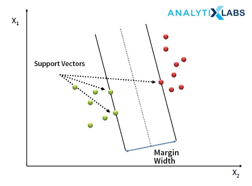
7. Support Vector Regression

Among the most sophisticated techniques of performing regression, Support Vector Regressors uses the concept of epsilon, whereby it can maximize the margin for the line of best fit, helping in reducing the problem of overfitting. SVR’s advantage over an OLS regression is that while they both come up with a straight line as a form of predicting values, thus solving only linear problems, SVR can use the concept of kernels that allows SVR to solve complicated non-linear problems.

Check this out to learn about Support Vector Machine Algorithm in Machine Learning

8. Poisson Regression

This type of regression is used when the dependent variable is countable values. Here the Y variable has a Poisson distribution. This form of regression can be considered an algorithm lying somewhere between linear and logistic regression.

9. Regularized Regression

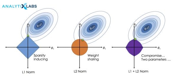
If the input data is suffering from multicollinearity, the coefficients calculated by a regression algorithm can artificially inflate, and features that are not important may seem to be important. To solve this problem, there is a concept of regularization where the features that are causing the problem are penalized, and their coefficient’s value is pulled down. There are multiple ways in which this penalization takes place. Some of them are the following:

1. Ridge   

Under Ridge Regression, we use an L2 regularization where the penalty term is the sum of the coefficients’ square. Here the value of the coefficient can become close to zero, but it never becomes zero.

2. Lasso

LassoRegression uses the L1 regularization, and here the penalty is the sum of the coefficients’ absolute values. The value of coefficients here can be pulled down to such an extent that it can become zero, renderings some of the variables to become inactive. This is the reason that Lasso is also considered as one of the feature reduction techniques.

3. Elastic Net

It is a combination of L1 and L2 regularization, while here, the coefficients are not dropped down to become 0 but are still severely penalized. The effect of the Elastic net is somewhere between Ridge and Lasso.

Linear Regression Line

The most important aspect f linear regression is the Linear Regression line, which is also known as the best fit line. When dealing with a dataset in 2-dimensions, we come up with a straight line that acts as the prediction. If the data is in 3 dimensions, then Linear Regression fits a plane. However, if we are dealing with more than 3 dimensions, it comes up with a hyper-plane.

To keep things simple, we will discuss the line of best fit. If we were to establish a relationship between one independent and a dependent variable, this relationship could be understood as Y = mx+c. The value of m is the coefficient, while c is the constant. To identify the value of m and c, we can use statistical formulas. Following is the method for calculating the best value of m and c –

            m = correlation between X and Y * (standard deviation of Y /     standard deviation of X)

            c = Mean of Y – (m *Mean of X)

Apart from this statistical calculation, as mentioned before, the line of best fit can be found by finding that value of m and c where the error is minimum. This is done by using optimization algorithms such as gradient descent, where the objective function is to minimize the sum of squared error (SSE).

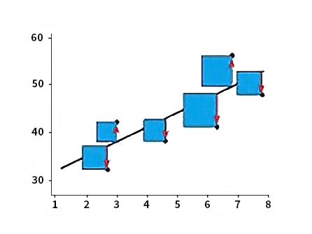
The Linear Regression line can be adversely impacted if the data has outliers. To accommodate those far away points, it will move, which can cause overfitting, i.e., the model may have a high accuracy in the training phase but will suffer in the testing phase.

Making Predictions

Once the line of best fit is found, i.e., the best value of m (i.e., beta) and c (i.e., constant or intercept) is found, the linear regression algorithm can easily come up with predictions. Here for a univariate, simple linear regression in machine learning where we will have an only independent variable, we will be multiplying the value of x with the m and add the value of c to it to get the predicted values.

However, Linear Regression is a much more profound algorithm as it provides us with multiple results that help us give insights regarding the data.

1. The most important use of Regression is to predict the value of the dependent variable. Here we can establish a relation between multiple X variables. For example, if we have 3 X variables, then the relationship can be quantified using the following equation-

Y = b1x1 + b2x2 + b3x3 + C

where,

b is the value of beta or coefficient

c is the value constant or intercept

• We can quantify the impact each X variable has on the Y variable. The coefficient can be read as the amount of impact they will have on the Y variable given an increase of 1 unit. For example, if we have X variable as customer satisfaction and the Y variable as profit and the coefficient of this X variable comes out to be 9.23, this would mean that the value for every unit increases in customer satisfaction of the Y variable increases by 9.23 units. This way, we can assess which variables have a positive and negative impact on the Y variable.

• Linear Regression also runs multiple statistical tests internally through which we can identify the most important variables. If the data is standardized, i.e., we are using the z scores rather than using the original variables. The value of coefficients becomes “calibrated,” i.e., we can directly look at the beta’s absolute value to understand how important a variable is. However, this is not true if we are using non-metric free variables. If our input variables are on different scales, then the absolute value of beta cannot be considered “weights” as these coefficients are “non-calibrated.”

To solve such a problem, Linear Regression runs multiple one sample t-tests internally where the null hypothesis is considered as 0, i.e., the beta of the X variable is 0. In contrast, the Alternative Hypothesis states that the coefficient of the X variable is not zero. This way, we take a clue from the p-value where if the p-value comes out to be high, we state that the value of the coefficient for that particular X variable is 0. The value we are seeing is statistically insignificant. Similarly, if we find the value of p to be lower than 0.05 or 0.1, then we state that the value of the coefficient is statistically significantly different from 0, and thus, that variable is important.

Once important variables are identified by using the p-value, we can understand their relative importance by referring to their t-value (or z-value), which gives us an in-depth understanding of the role played by each of the X variables in predicting the Y variable.

Therefore, running a linear regression algorithm can provide us with dynamic results, and as the level of interpretability is so high, strategic problems are often solved using this algorithm.

Frequently Asked Questions

To summarize the various concepts of Linear Regression, we can quickly go through the common questions regarding Linear Regression, which will help us give a quick overall understanding of this algorithm.

What is the linear regression algorithm?

It is a statistical, linear, predictive algorithm that uses regression to establish a linear relationship between the dependent and the independent variable. It comes up with a line of best fit, and the value of Y (variable) falling on this line for different values of X (variable) is considered the predicted values.

What is the objective of the simple linear regression algorithm in machine learning?

A simple linear regression algorithm in machine learning can achieve multiple objectives. Firstly, it can help us predict the values of the Y variable for a given set of X variables. It additionally can quantify the impact each X variable has on the Y variable by using the concept of coefficients (beta values). Lastly, it helps identify the important and non-important variables for predicting the Y variable and can even help us understand their relative importance.

What are the four assumptions of linear regression?

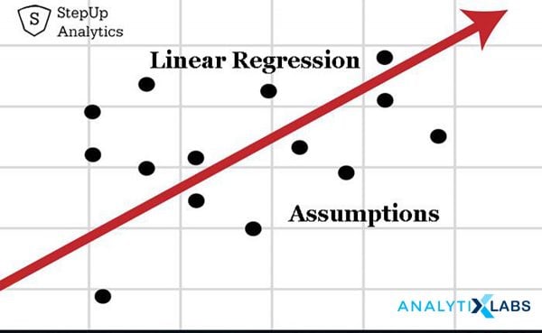
Being a statistical algorithm, unlike other tree-based and some other Machine Learning algorithms, Linear Regression requires a particular set of assumptions to be fulfilled if we wish it to work properly. Among the numerous assumption, the four main assumptions that we need to fulfill are as follows-

1. The relationship between the dependent and independent variables should be linear. In simple words, if we calculate the correlation between the X and Y variable, then they should have a significant value of correlation among them as only then we can come up with a straight line that will pass from the bulk of the data and can acts as the line for predictions. Note that this relationship can be either negative or positive but should be a strong linear relationship.
2. The models suffer from the problem of overfitting, which is the model failing in the test phase. This happens due to the problem of multicollinearity. The data is said to be suffering from multicollinearity when the X variables are not completely independent of each other. Thus the assumption is that all the X variables are completely independent of each other, and no X variable is a function of other X variables.
3. It is presumed that the data is not suffering from Heteroscedasticity. A dataset has homoscedasticity when the residual variance is the same for any value of the independent variables. If this not the case, it can mean that we are dealing with different types of data that have been combined. If this variance is not constant throughout then, such a dataset can not be deemed fit for running a linear regression,
4. The last assumption is that the dependent variable is normally distributed for any independent variable’s fixed value. This is especially important for running the various statistical tests that give us insights regarding the relationship of the X variables having with the Y variable, among other things. If the Y variable is not normally distributed, transformation can be performed on the Y variable to make it normal.

To summarize the assumption, the correlation between the X and Y variable should be a strong one. The correlation between the X variables should be weak to counter the multicollinearity problem, and the data should be homoscedastic, and the Y variable should be normally distributed. In addition to this, we should also make sure that no X variable has a low coefficient of variance as this would mean little to no information, the data should not have any missing values, and lastly, the data should not be having any outliers as it can have a major adverse impact on the predicted values causing the model to overfit and fail in the test phase.

How to Implement Linear Regression in Python

The implementation of linear regression in python is particularly easy. We first have to take care of the assumptions, i.e., apart from the four main assumptions, ensure that the data is not suffering from outliers, and appropriate missing value treatment has taken place. Once all of this is done, we also have to make sure that the input data is all numerical as for running linear regression in python or any other language, the input data has to be all numerical, and to accomplish this, the categorical variables should be converted into numerical by using the concept of Label Encoding or One Hot Encoding (Dummy variable creation).

After preparing the data, two python modules can be used to run Linear Regression. One is statsmodels while the other is Sklearn. While both provide accurate results, statsmodels implement linear regression in a more statistical way providing us detailed reports regarding the various statistical tests ran by it internally. This helps us in identifying the relative importance of each independent variable. Sklearn, on the other hand, implements linear regression using the machine learning approach and doesn’t provide in-depth summary reports but allows for additional features such as regularization and other options.

Following are the sample codes for running linear regression in python using the above-mentioned modules:

1. statsmodels

Importing important modules

>>
import statsmodels.formula.api as sm

>> import numpy as np

>> import pandas as pd

Importing the dataset

>> df = pd.read_excel(dataset.xlsx')

Initialization of the model

>> model = sm.ols(Y~X1+X2+X3, data=df)

Fitting the model on the dataset

>> model = model.fit()

Coming up with the model summary

>> print(model.summary())

Coming up with predictions

>> model.predict(df)

2. sklearn

Importing sklearn library

>> import sklearn

Diving the dataset in train and test

(if required, the data can also be divided into X and Y as for Sklearn, the dependent and the independent variable are be saved separately)

>>
from sklearn.model_selection import train_test_split

>>
train_X, test_X, train_y, test_y = train_test_split( df[“X1”,”X2”,”X3”] ,df[“Y”],
test_size = 0.2, random_state = 123 )

Importing the module for running linear regression using Sklearn

>>
from sklearn.linear_model import LinearRegression

Initializing and Fitting the model

>>
linreg = LinearRegression()

>>
linreg.fit( train_X, train_y )

Finding coefficient and intercept values

>>
linreg.coef_[0]

>>
linreg.intercept_

Predicting the values of the test dataset

>> linreg.predict(test_X )

The practical implementation of linear regression is straightforward in python. There is little difference in the implementation between the two major modules; however, each has its own advantages.

Linear Regression is the stepping stone for many Data Scientist. This algorithm uses a rather simple concept of a linear equation and uses a straight-line formula to develop many complicated and important solutions. While being a statistical algorithm, it faces having the data in proper assumptions and having a less powerful predictive capability when the data is in high dimensions. However, all these aspects are overshadowed by the sheer simplicity and the high level of interpretability. Lastly, one must remember that linear regression and other regression-based algorithms may not be as technical or complex as other machine learning algorithms. Still, their implementation, especially in the machine learning framework, makes them a highly important algorithm and should be explored at every opportunity.

You may also like to read: How to Choose The Best Algorithm for Your Applied AI & ML Solution.