There are numerous aspects of the data science world that have predictive models at their core. A good model is directly dependent on the correct choice of algorithm that a data scientist selects. However, data scientists often find it difficult to pick the right algorithm because there are numerous of them. To make an informed decision, the decision tree algorithm plays a pivotal role. This article will go over the advantages and disadvantages of decision tree algorithm in machine learning.
What is a Decision Tree Algorithm?
A data scientist evaluates multiple algorithms to build a predictive model. One such algorithm is the decision tree algorithm. It is a non-parametric supervised learning algorithm and is hierarchical in structure. Like a tree, it has root nodes, branches, internal nodes, and leaf nodes.
Features and Characteristics
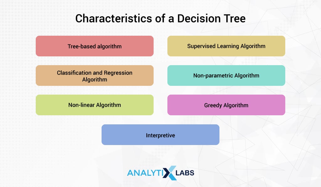
The decision for choosing an algorithm depends on various factors. Any algorithm in data science and machine learning is categorized and labeled in multiple ways based on its characteristics. Same applies to the decision tree algorithm. Below are the features and characteristics of the decision tree algorithm.
It is a tree-based algorithm
Algorithms are categorized based on the discipline of study they involve. For example, there are statistical, distance-based, neural-based, etc. algorithms.
Supervised Learning Algorithm
Decision Tree works in a supervised learning setup. This means that the data set required by the algorithm needs to have a dependent variable (Y variable) that is predicted by understanding its relationship with the various independent variables (X variables/predictors).
Classification and Regression Algorithm
An exciting aspect of the Decision Tree is that it can solve both classifications and regression problems . Classification algorithms can predict categorical variables, whereas regression algorithms predict continuous variables. The decision tree can also solve multi-class classification problems also (where the Y variable has more than two categories).
Non-linear Algorithm
Decision Tree creates complex non-linear boundaries, unlike algorithms like linear regression that fit a straight line to the data space to predict the dependent variable.
Greedy Algorithm
It’s a characteristic that is better aligned with the concept of splitting. To put it simply, the decision tree doesn’t think long-term and is ‘short-sighted’ when looking for a solution . This feature has its advantage and disadvantages.
Interpretive
Algorithms can either be interpretive or can act as a black box. Decision tree, somewhat like Linear Regression and unlike Neural Networks, is interpretive. This means one can interpret how the algorithm came up with the prediction.
How does Decision Tree Work?
To properly understand how decision trees work, you must understand the concepts like different types of nodes, splitting, pruning, attribute selection methods, etc. However, before getting technical, let’s first intuitively understand how a decision tree works with an example.
Let’s say you are an underwriter responsible for accepting or rejecting a loan application. Now you come across a loan application, and you gained the following information from the documents provided by the applicant-
- Gender: Male
- Income: $56,000
- Service Type: Salaried
- Marital Status: Single
- Height: 1.66 cm
- Eye Color: Green
Now, to decide whether to grant the loan or not, you need to know how likely the applicant is to default. To do so, you look at the historical data of the loans granted by the bank and their eventual outcome (default or repaid). You slice and dice the data and work in a step-by-step manner.
Step 1:
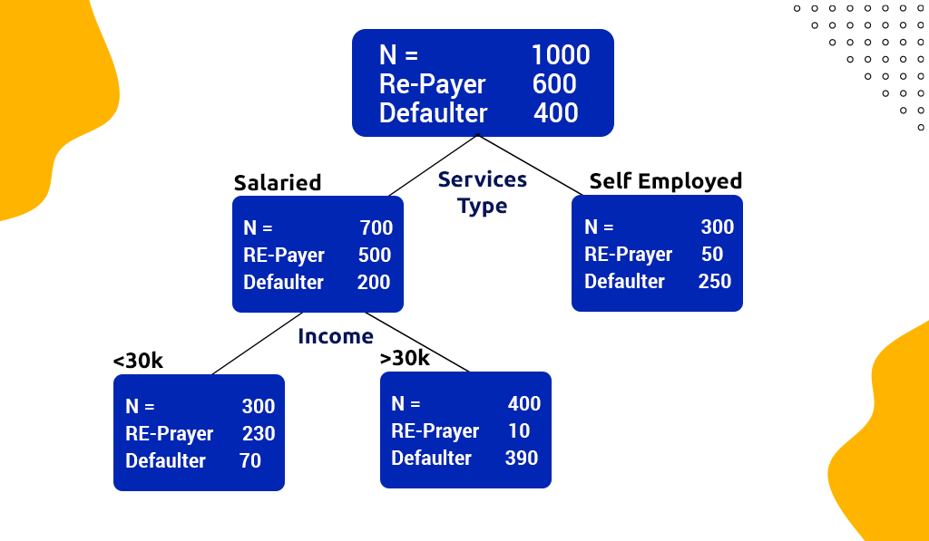
In the data, you find 1,000 observations, out of which 600 repaid the loan while 400 defaulted. After many trials, you find that if you split the data on the service type, you get two groups.
- The group where the service type is salaried has 700 observations, with 500 observations having repaid the loan and 200 being defaulted. On the other hand, where the service type was self-employed, out of 300, only 50 repaid the loan while the remaining 250 defaulted. Therefore, by using this attribute to ‘split’ the data; you created ‘pure’ or homogeneous ‘groups,’ i.e., where there was an overwhelming concentration of one of the class labels.
- A perfect ‘pure’ group is one where in the salaried group, all the observations are of those people who’ve repaid their loans and all self-employed by default. Similarly, an impure node is where both the groups had an equal number of defaulted and repaid observations.
Step 2:
You yet again slice and dice the data and find that if you further split the ‘salaried group’ (having 700 observations) using the attribute ‘income’, you get a good result. Here, if the individual’s Income is less than $30,000, then there are 300 observations with 230 being re-payers and 70 being defaulters. When the Income is above $30,000, there are 400 observations with 10 re-payers and 390 defaulters.
Step 3:
After further analysis, you find another attribute to split the above-mentioned Income>30,000 group. This time it’s the eye color. Individuals with green eye color were 20, with only 1 being a re-payer and 19 being defaulters, and among the individuals with non-green eye color, 229 re-payers and 51 being defaulters.
However, you realize that eye color doesn’t make sense in deciding whether to grant a loan or not and feel that you are ‘overanalyzing’ the patterns in the data.
Step 4:
Since you don’t find any other attribute that provides you with homogeneous groups, you stop at this juncture. Now, you can summarize your findings in the form of rules-
- Self Employed: Probability of default = 0.83 (250/300)
- Salaried & Income>$30K: Probability of Default = 0.23 (70/300)
- Salaried & Income<$30K: Probability of Default = 0.98 (390/400)
Decision Tree works similarly.
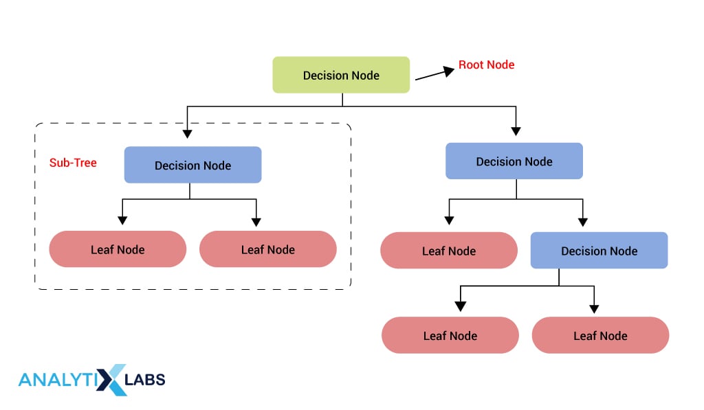
Here the first group that we start splitting is known as the Root Node, the group that is further split after the root node is known as the decision node, and the group that is not split and is used to make the predictions (or come up with probabilities as done above i.e. is involved in producing the decision rules) is known as the leaf node.
This whole structure is known as a decision tree while a sub-structure is known as a sub-tree, and the process of dividing the groups is known as splitting.
The next question is: How do you conclude which attribute to split the data/node? This is where you must learn about attribute selection and the various mechanisms involved.
Attribute Selection
Different decision tree algorithms use different methods to select the attribute to split a node. As discussed above, the idea is to get a pure, i.e., homogeneous node upon splitting.
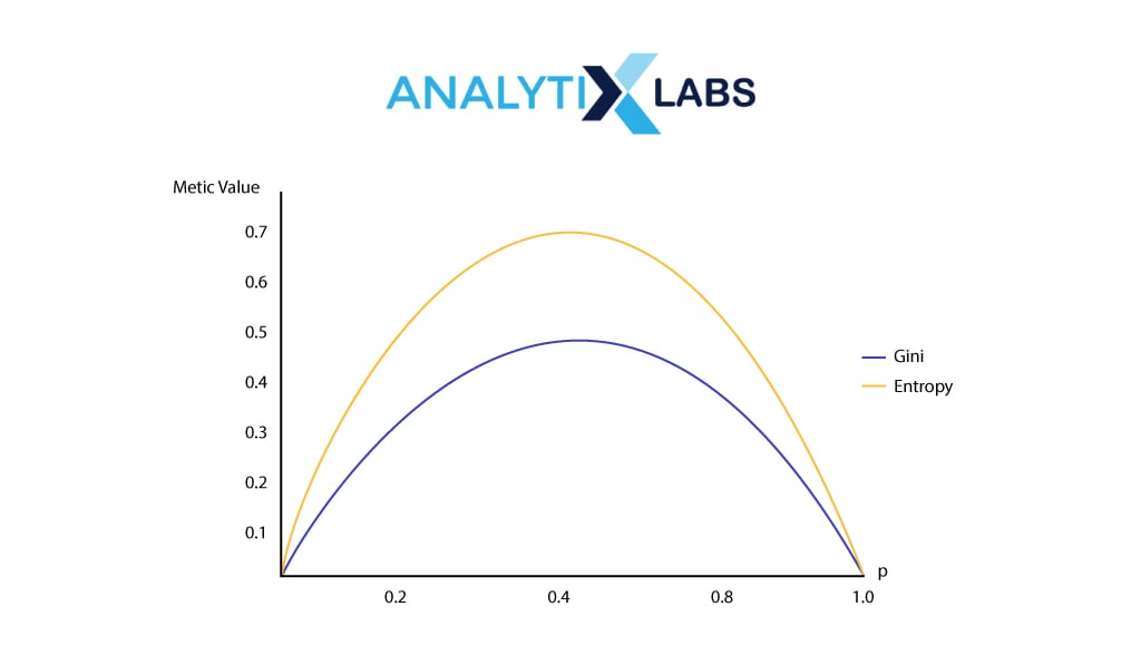
While there are many methods, the following are the most common methods of attribute selection.
-
Entropy
Entropy is a common phenomenon in physics that refers to the level of order in a system. Entropy is used in Decision Tree Classifiers to find how ‘orderly,’ i.e., homogeneous the node is upon splitting. The formula of Entropy is-
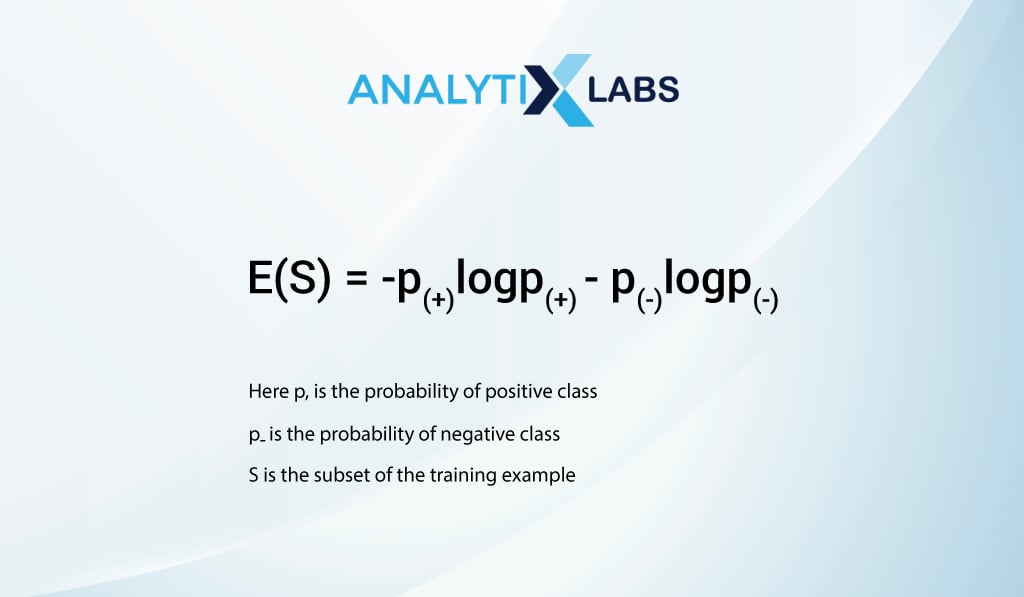
A lower value means that the split provides a purer node.
-
Information Gain
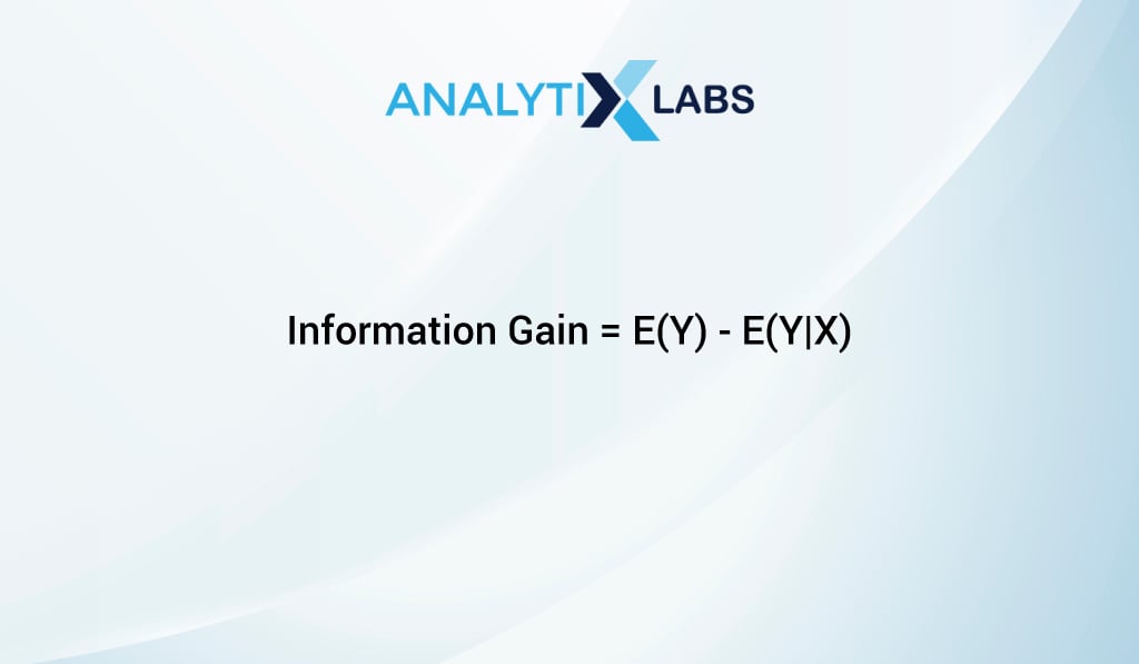
Information Gain is related to Entropy, and it is calculated by subtracting the Entropy provided by an attribute from the Entropy of the complete data. This difference is the ‘gain’ and should be maximized.
-
Gain Impurity
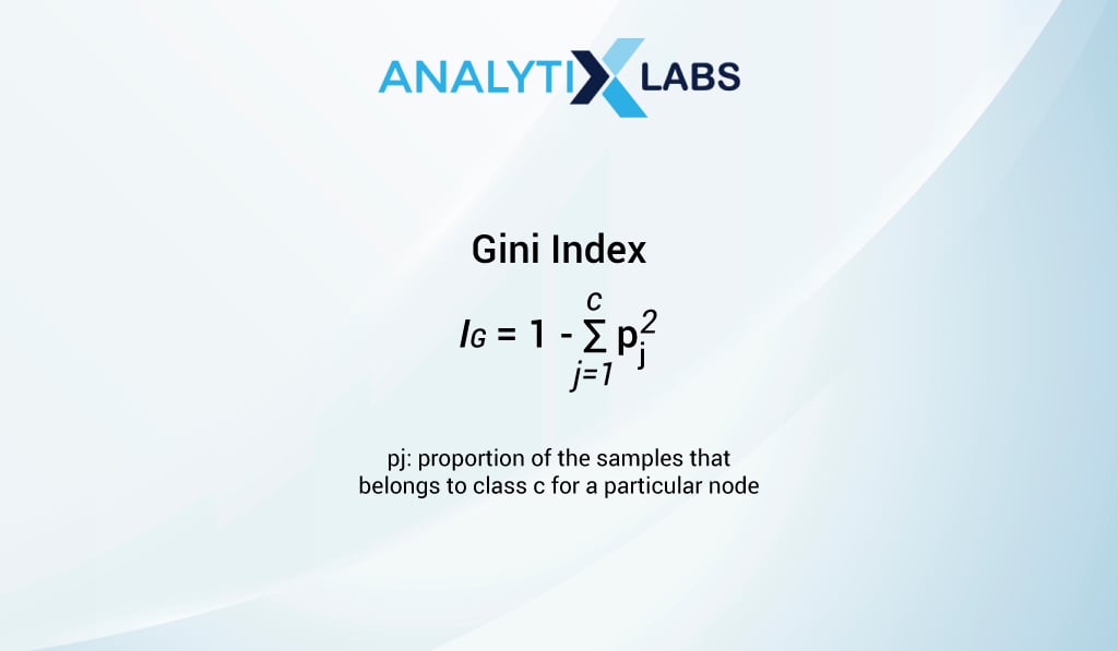
Another critical method used in decision tree classifier is Gini impurity (sometimes referred to as Gini index) which calculates the likelihood of some data being misclassified if it was provided by a random class as per the class distribution in the dataset. Its value is between 0 and 0.5, which indicates a split’s impurity, and therefore a lower value is better.
-
Chi-Square
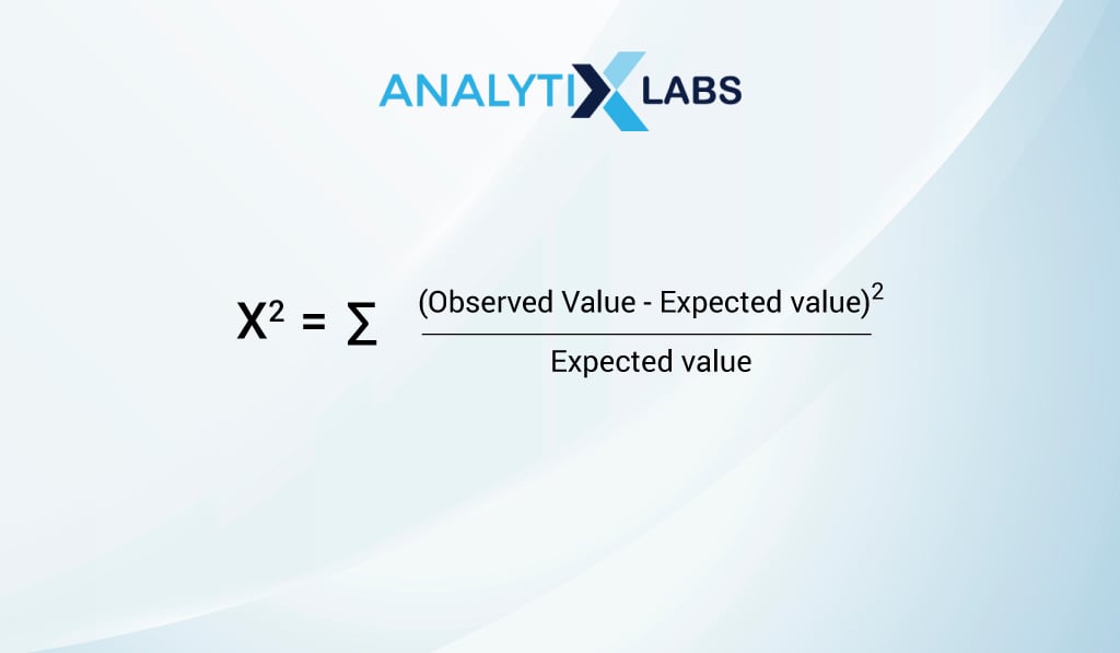
A common non-parametric statistical test, chi-square, is used to understand the relationship between two categorical variables. Here a high chi-square value means that the attribute affects the Y variable making the feature significant for being used for splitting a node.
If you are wondering how independent numerical variables are used for splitting, then you must know that the decision tree algorithm uses a brute force method where it creates binary splits of the numerical variable and checks each combination purity.
-
ANOVA
ANOVA is another statistical test and is used when dealing with regression problems. Here a larger f-value indicates a better split.
Parameters
Dealing with parameters is part of the advantages and disadvantages of decision trees.
If you read the above-discussed intuitive understanding of decision again, you will realize two possible scenarios.
When done manually, you can either not consider too many features for coming up with the rules or can go overboard in analyzing the data and find patterns that are just unique to the dataset (and end up creating a highly complex decision rule as was going out be the case if we would have included eye color in our decision making).
The decision tree faces a similar problem. Not using too many rules, i.e., by creating a shallow tree, the model can underfit and not learn the relevant patterns. On the other hand, if we create a highly deep tree, then we will end up overfitting the model, i.e., we will learn patterns in data that were unnecessary and were not supposed to be discovered.
This trade-off of high bias (underfitting) and high variance(overfitting) can be balanced by controlling splitting or the tree’s depth and consequently the number of leaf nodes. To control the depth, you can control splitting, a top-down approach where you control various parameters splitting off the nodes. Alternatively, you can perform pruning, a bottom-up approach where less important nodes are removed.
Standard parameters of splitting are the following-
-
Max Depth
The maximum depth of trees allowed
-
Minimum Samples Split
The minimum number of observations required in a node to be allowed for a split
-
Min Samples Leaf
The minimum number of observations allowed in a leaf node
-
Max Features
The maximum number of features allowed for splitting the nodes
Advantages and Disadvantages of Decision Tree
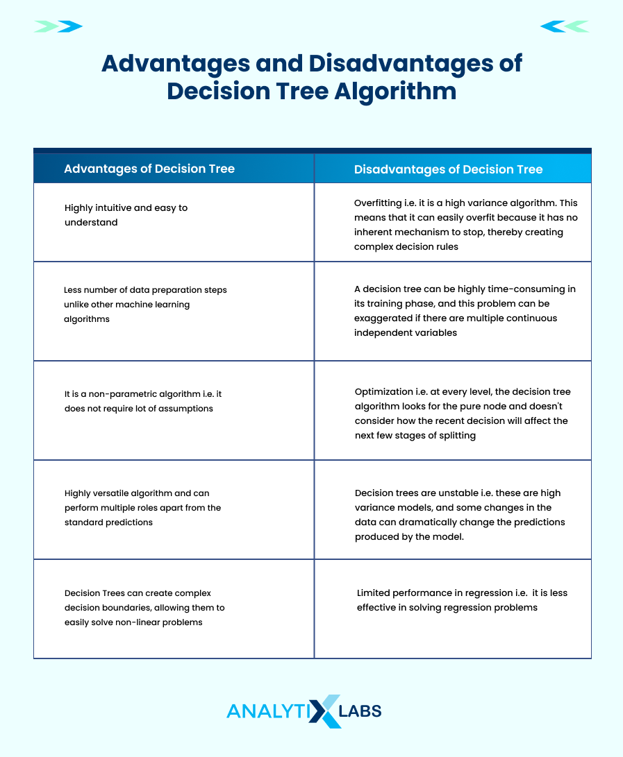
Now, as you understand how the algorithm works, let’s move on to the advantages and disadvantages of decision trees.
Advantages of Decision Trees
A decision tree is often the algorithm that data scientists start with due to its various features. Following are the decision tree advantages.
-
Interpretability
One of the most significant Decision tree advantages is that it is highly intuitive and easy to understand. Also, the rules implemented by decision trees can be displayed in a flow chart-like manner, allowing data scientists and other professionals to explain to the stakeholders the model’s predictions.
This induces confidence in the stakeholders and provides detailed information about what is happening and why it is happening. Thus unlike other algorithms, it is easy to interpret, visualize and comprehend.
-
Less Data Preparation
A major hurdle when developing a model involving other algorithms is data preparation. This is because any model works on the ‘garbage in garbage out‘ principle, i.e., the quality of the predictions made by the model is dependent upon the quality of data being fed to the model to train on , and this is where decision trees have an edge.
Typical data preparation steps such as data normalization/standardization, missing value treatment, outlier capping, etc., are not required for the decision tree, making it a ‘go-to’ algorithm for data scientists.
-
Non-Parametric
Algorithms like linear regression, naïve Bayes, etc., require a lot of assumptions that need to be fulfilled for the model to work effectively. Decision Trees, as explained earlier, is a non-parametric algorithm, and thus there are no significant assumptions to be fulfilled or data distribution to be considered.
-
Versatility
Another decision tree advantage is that it’s a highly versatile algorithm and can perform multiple roles apart from the standard predictions.
This includes its capability to perform data exploration, using it as a baseline model for quick understanding of data quality, etc. On top of this, a decision tree can solve regression as well as classification problems, and variants of it can also work on segmentation problems.
-
Non-Linearity
Decision Trees can create complex decision boundaries, allowing them to easily solve non-linear problems. While other algorithms can solve the non-linear problem, the advantage of the Decision Tree is that it offers interpretability.
Disadvantages of Decision Tree
There are several disadvantages of decision trees that make them less valuable or restrict their use in many cases. Following are the most prominent disadvantages of decision trees.
-
Overfitting
Among the most common and prominent disadvantages of decision trees are that it’s a high variance algorithm. This means that it can easily overfit because it has no inherent mechanism to stop, thereby creating complex decision rules. As discussed before, various parameters can be tuned to control the splitting process, or pruning can be performed, but its effectiveness can be limited.
-
Feature Reduction & Data Resampling
A decision tree can be highly time-consuming in its training phase, and this problem can be exaggerated if there are multiple continuous independent variables. Also, if there is an imbalanced class dataset, the model can become biased towards the majority class. Therefore there is a need to work on the rows as well as the column of the dataset.
- Firstly, you need to reduce the number of features so that the time complexity can be reduced.
- Secondly, the rows might need to be duplicated or removed to perform resampling to resolve the class imbalance issue.
-
Optimization
At every level, the decision tree algorithm looks for the pure node and doesn’t consider how the recent decision will affect the next few stages of splitting. This is the reason that it is known as a greedy algorithm.
This heuristic method of working makes the model interpretable but doesn’t ensure that the algorithm will return the globally optimal result. Also, if a few variables are highly significant or cause data leakage, they will ‘hijack’ the process. All these issues can be resolved by using an ensemble of decision trees, but that results in a complete loss of interpretability.
All these advantages and disadvantages of decision trees must be kept in mind when deciding on the algorithm to build a model as you can achieve better results by making an informed decision.
Benefits of Decision Tree
Having discussed the advantages and disadvantages of decision tree, let us now look into the practical benefits of using decision tree algorithm.
- Solves strategic Problem:One of the significant benefits of decision trees is that it helps solve strategic problems. It’s because of the high interpretability of decision trees. For example, when exploring and solving fundamental issues such as looking for growth and expansion opportunities, profit maximization, reducing cost, etc. Here decision trees can be used to look at the historical data and find patterns to understand what factors affect sales etc.
- Supports in Non-predictive aspects:Decision Tree not only helps create a predictive model but can also be used in other model-building aspects. For example, Decision tree can be used for feature selection as it identifies the important variable in the process. Understanding decision trees enables you to use various other tree-based algorithms involved in unsupervised learning that help in anomaly or outlier detection, reducing data space, etc.
Limitations of Decision Tree
Like all algorithms, decision tree algorithm has several limitations [along with the listed disadvantages of decision tree algorithm].
-
Unstable
Decision trees are high variance models, and some changes in the data can dramatically change the predictions produced by the model. This issue makes it difficult to be used data that is dynamic and can change over a period of time.
Therefore, despite the advantages and disadvantages of decision trees, a significant limitation is that they cannot be used over long periods and are highly susceptible to data drifts. To resolve this, other tree-based algorithms such as random forest or various boosting algorithms can be used, but as mentioned above, they lose interpretability.
-
Limited Performance in Regression
Another major limitation of decision trees is that it is less effective in solving regression problems. Certain types of decision tree algorithms lose essential information and are computationally expensive when dealing with numerical dependent variables.
Endnotes
Decision tree algorithm is one of the most popular algorithms used for predictive modeling. It is robust in nature. Despite all the limitations and disadvantages of decision tree, it is still accurate in terms of splitting the data and creating a predictive model.

