How Data Reduction Can Increase the Efficiency in Data Mining?

We are generating petabytes of data in a click. Everything acts like a touchpoint – be it the price of toothpaste or asking Google Maps for direction. We keep creating a pipeline of data, one on top of another. Thanks to the speed at which data is growing, we need to understand the means to combat the “space” that this data is taking up. Data reduction in data mining can help in pre-processing and handling of this large data set.

In this article, we will understand what is data reduction in data mining, explore data reduction in data mining, and how data reduction is important for data compression.

Also read: How Data Compression Technique helps in Data Representation?

There are three basic techniques for data reduction in data mining:

1. Dimensionality reduction
2. Numerosity reduction
3. Data compression

We will look at each of these in detail, along with explaining the concept of data reduction, and data compression in data mining. Let’s get started. 

What is Data Reduction?

Data reduction involves reducing a large capacity of the data into small datasets. The goal of data reduction is to present and define the data in a concise manner. 

In a nutshell:

Data reduction helps in lowering costs and increasing storage efficiency.

What is Data Reduction in Data Mining? 

The data that is generated is not clean, nor is it small or has less data. The datasets are usually voluminous, having zettabytes of data. In such cases, a lot of time goes into processing, applying the data mining tools, and even running complex queries – making it impractical to work with such data. Here’s how data is processed:

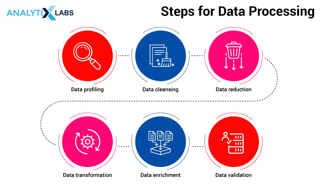
In the data processing steps, there is an important step of data reduction without which data processing is incomplete. Without data reduction in place, it can become extremely tedious to manage the huge data. The mishandling of data directly impacts data validation, which is the final step in the data processing.

Data reduction is a mechanism to reduce the data volume while maintaining the integrity of the data. 

Data Reduction Methods

(1) Data Cube Aggregation

Data Cube Aggregation in data mining represents the data in cube format by performing aggregation on data. In this data reduction technique, each cell of the cube is a placeholder holding the aggregated data point. This cube stores the data in an aggregated form in a multidimensional space. The resultant value is lower in terms of volume i.e. takes up less space without losing any information.

Here’s an example of the data cube aggregation methodology [Data sourced from Tutorials Point]

Below we have the quarterly sales data of a company across four item types: entertainment, keyboard, mobile, and locks, for one of its locations aka Delhi. The data is in 2-dimensional (2D) format and gives us information about sales on a quarterly basis.

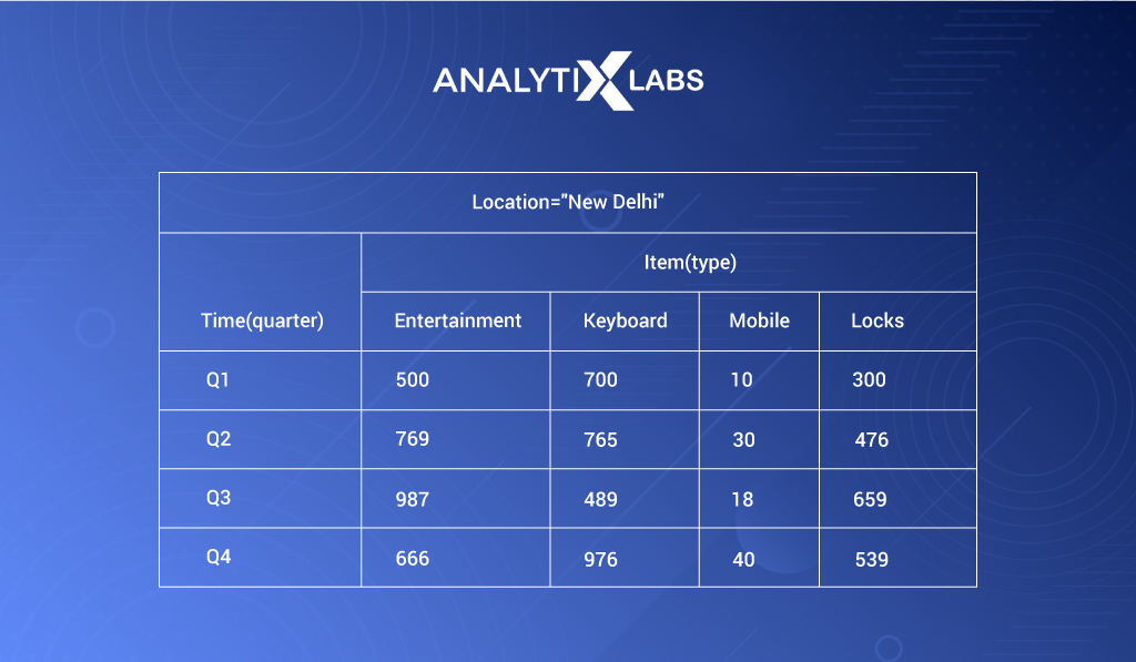
Viewing 2-dimensional data in the form of a table is indeed helpful. Let’s say we increase one more dimension and add more locations in our data – Gurgaon, Mumbai, along with the already available location, Delhi, as below: 

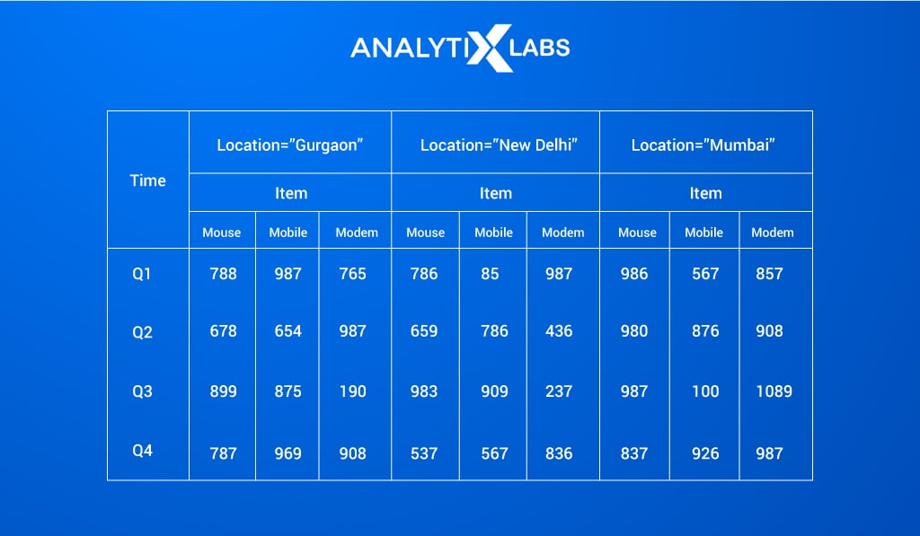
Now, rather than viewing this 3-dimensional data in a tabular structure, representing this data in a cube format increases the readability of the data:

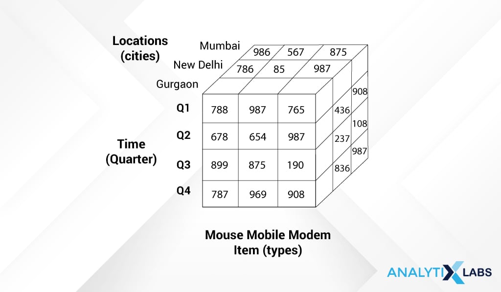
Each side of the cube represents one dimension- Time, Location, and Item Type (Mouse mobile modem).

Another usability of the data cube aggregation in data mining is when we want to aggregate the data values. In the example below, we have quarterly sales data for different years from 2008 to 2010 [Data sourced from Binary Terms]

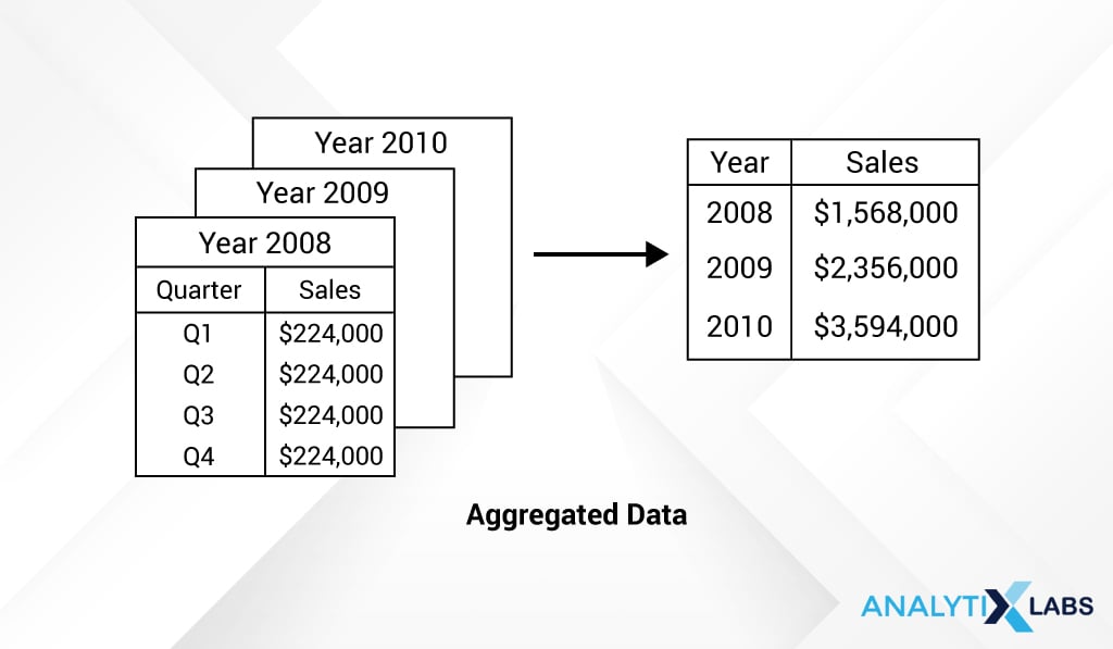
However, to make an analysis of any sort, we typically work with annual sales. So, can visually depict the yearly sales data by summing over the sales amount across other dimensions like below:

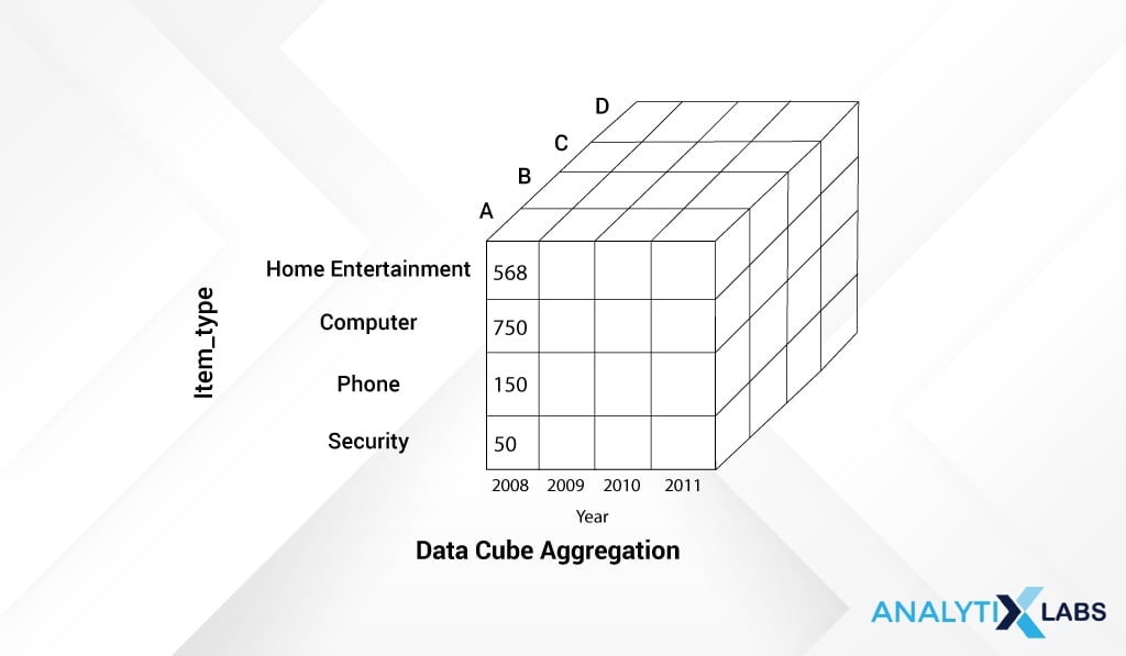
Data cube aggregation in data mining is useful for storing and showing summarized data in a cube form.

Here, data reduction is achieved by aggregating data across different levels of the cube. It is also seen as a multidimensional aggregation that enhances aggregation operations.

In short:

Data aggregation is a very simplistic way of representing data in a summarized manner.

(2) Data Compression

Data compression in data mining as the name suggests simply compresses the data. This technique encapsulates the data or information into a condensed form by eliminating duplicate, not needed information. It changes the structure of the data without taking much space and is represented in a binary form.

There are two types of data compression:

1. Lossless Compression: When the compressed data can be restored or reconstructed back to its original form without the loss of any information then it is referred to as lossless compression.
2. Lossy Compression: When the compressed data cannot be restored or reconstructed back into its original form then referred to as Lossy compression.

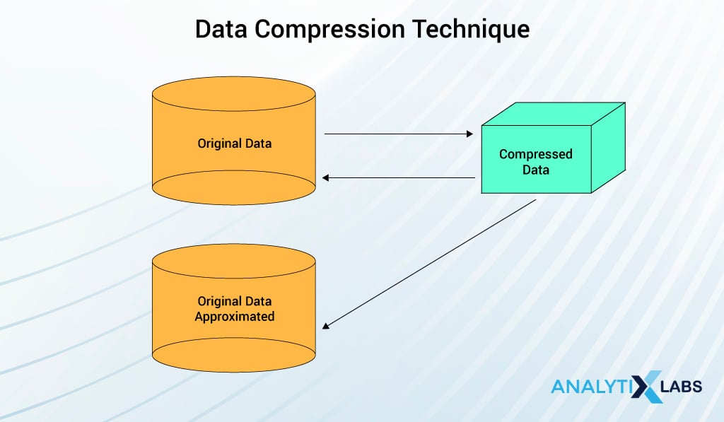
Data compression technique varies based on the type of data.

1. String data:  In string compression, the data is modified in a limited manner without complete expansion; hence the string is mostly lossless as the data can be retrieved back to its original form. Therefore it is lossless data compression. There are extensive theories and well-tuned algorithms that are used for data compression. 
2. Audio or video data: Unlike string data, audio or video data cannot be recreated to its original shape, hence is lossy data compression. At times, it may be possible to reconstruct small bits or pieces of the signal data but you cannot restore it to its whole form.
3. Time Sequential data:  The time-sequential data is not audio data. It is by large, usually short data fragments and it varies slowly with time as is used for data compression.

Data Compression Methodologies

There are two methodologies:

1. Dimensionality 
2. Numerosity reduction

(1) Dimension reduction

In the language of data,  dimensions are also known as features or attributes . These dimensions are nothing else but properties of the data, i.e., describing what the data is about.

For instance, we have the data of employees of a company. We have their name, age, gender, location, education, and income. All these variables do nothing but help us to know, understand and describe the data point. 

As the features increase, the sparsity of the dataset also increases. The sparsity indicates that there is a relatively higher percentage of the variables that do not contain actual data. These “empty” cells or NA values take up unnecessary storage.

Dimensionality Reduction in data mining is the process of reducing the data by removing these features from the data. There are three techniques for this: 

• Wavelet Transformation
• Principal Component Analysis- PCA in data mining
• Feature Selection or Attribute Subset Selection

1. Wavelet Transformation in Data Mining

Wavelet Transform in Data Mining is a form of lossy data compression.

Let’s say we have a data vector Y, by applying the wavelet transform on this vector Y, we would receive a different numerical data vector Y’, where the length of both the vectors Y and Y’ are the same. Now, you may be wondering how transforming Y into Y’ helps us to reduce the data. This Y’ data can be trimmed or truncated whereas the actual vector Y cannot be compressed. 

Let’s say we have a data vector Y. When we apply wavelet transformation on this vector Y, we get a different numerical data vector Y’ where the length of both the vectors Y and Y’ are the same now.

The reason it is called ‘wavelet transform’ is that the information here is present in the form of waves, like how a frequency is depicted graphically as signals. The wavelet transform also has efficiency for data cubes, sparse or skewed data. It is mostly applicable for image compression and for signal processing.

2. Principal Component Analysis (PCA)

Principal component analysis – PCA in data mining, a technique for data reduction in data mining, groups the important variables into a component taking the maximum information present within the data and discards the other, not important variables. 

Now, let’s say out of total n variables, k are such variables that are identified and are part of this new component. This component is now what is representative of the data and used for further analysis. 

In short,  PCA in data mining is applied to reducing multi-dimensional data into lower-dimensional data.  This is done by eliminating variables containing the same information as provided by other variables and combining the relevant variables into components. The principal component analysis is also useful for sparse, and skewed data.

3. Feature Selection or Attribute Subset Selection

The attribute subset selection or feature selection method decreases the data volume by removing unnecessary variables. Hence, the name feature selection.  This is done in such a way that the probability distribution of the reduced data is similar to that of the actual data, given the original variables.

(2) Numerosity reduction

Another methodology in data reduction in data mining is numerosity reduction in which the volume of the data is reduced by representing it in a lower format. There are two types of this technique: parametric and non-parametric numerosity reduction. 

1. Parametric Reduction

The parametric numerosity reduction technique holds an assumption that the data fits into the model. Hence, it estimates the model parameters, and stores only these estimated parameters, and not the original or the actual data. The other data is discarded, leaving out the potential outliers.

The ways to perform parametric numerosity reduction are: Regression and Log-Linear. Both the parametric methods of regression and log-linear methods are applicable for sparse and skewed data.

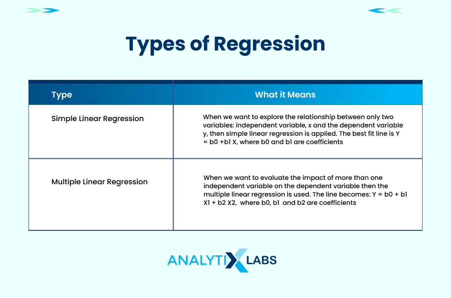
• Regression: Linear Regression analysis is used for studying or  summarizing the relationship between variables that are linearly related. The regression is also of two kinds: Simple Linear regression and Multiple Linear regression.

• Log-Linear: This technique is useful when the purpose is to explore and understand the relationship between two or more discrete variables. For understanding purposes, let’s take a scenario where in n-dimensional space, a set of tuples (‘apple’, ‘banana’, ‘cherry’, ‘dragon fruit’) is available. Now, we can get the joint probabilities of this tuple by taking the product of these marginal elements in the following way:

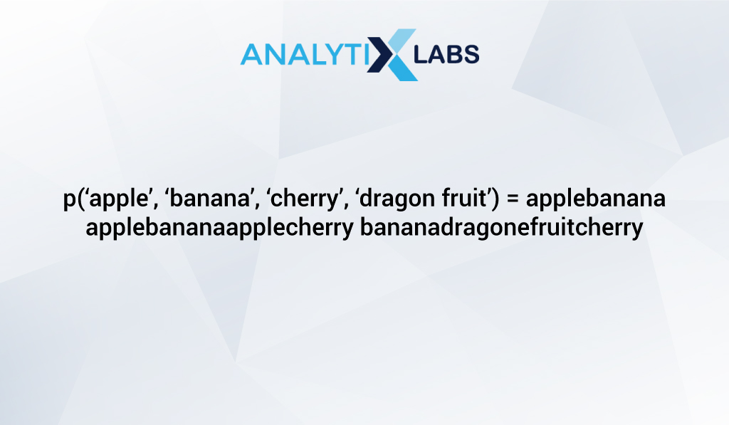
This way the log-linear model can be used for studying the probability of each of these tuples in this multi-dimensional space.

2. Non-parametric Reduction

On the other hand, the non-parametric methods do not hold the assumption of the data fitting in the model. Unlike the parametric method, these methods may not give a very high decrease in data reduction though it generates homogenous and systematic reduced data in spite of the size of the data.

The types of Non-Parametric data reduction methodology are:

• Histogram 
• Clustering
• Sampling 

(3) Discretization & Concept Hierarchy Operation

Data discretization methodology  minimizes large continuous data points into smaller fixed sets of data points . This data reduction can be achieved by dividing into a range of intervals with less loss of data. Now, for these interval data points, class labels or information can be used for replacing the original data values.

The process of discretization in data mining can be carried off on a recursive basis on an attribute leading to splitting of the values in a hierarchical or multiresolution manner. During the recursive process, the data is sorted at every step. This data reduction technique is faster when there are fewer unique values for sorting.  This partitioning of the data values is also known as concept hierarchy.

The data discretization techniques are sub-divided into following forms based on the application of class data: 

• Supervised discretization in data mining: In supervised discretization, class data or information is used.
• Unsupervised discretization in data mining: In unsupervised discretization, here the class data or information is not used.

These branching out of the  data discretization methodologies are on the basis of whether the class data or information is used or not. The unsupervised discretization further works on a strategy of how the data is split up (top-down) or merged (bottom-up). 

Subdivision of the data discretization is based on the following: 

• Top-down Discretization

In general, the top-down approach starts from the top and goes till the bottom of the ladder. In the top-down discretization, the splitting process starts by considering some breakpoints at the top and continues till the end for splitting the complete range of all the attributes.

• Bottom-up Discretization

The bottom-up discretization has the reverse mapping. It begins from the bottom and moves up the ladder to the top element of the series. Here, in the bottom-up discretization, all the continuous data values are taken as the prospective break points. Some of these points are discarded after being merged with the neighborhood data values. This is done so as to form the intervals.  

The concept hierarchy is similar to the concept of hierarchy that we know. Hierarchy means “a system or an organization that has many levels from the lowest to the highest. Here,  the data is numerically continuous in nature .  With these two understanding of what hierarchy is and the kind of data we have, let’s understand what it means for us from the point of data reduction. 

The concept hierarchy operation for a given numerical feature is defined as the reduction or discretization of this feature. These concept hierarchies for numerical features can be automatically or dynamically created given the analysis of the data distribution.

 It is conducted by iteratively lowering the data by collecting and replacing the low-level concepts (such as numerical values for the feature age) by higher-level concepts (such as young, middle-aged, or senior). The concept hierarchy basically can be seen by labeling a series of values which are of a general concept to a specialized concept. 

The methodologies for concept hierarchy operation are:

• Histogram Analysis 
• Binning 
• Cluster Analysis
• Entropy-Based Discretization 
• Data Segmentation by natural partitioning
• Interval merging by Chi^2 Analysis

End-notes:

The basis of any data reduction in data mining and warehousing is of reducing the data and representing the data in a lower-dimensional space. The data reduction in data mining is not only about reducing features via Principal Component Analysis – PCA in data mining or by matrix factorization.

There are far more procedures and methodologies available for reducing data. We hope this article was useful to explain the concept of data reduction, getting to know the various data reduction techniques in data mining, understanding data reduction in data mining and data warehousing, and how data reduction can be achieved by these methodologies.