Application of Central Limit Theorem in Supply Chain: An Illustration

You are far from being called a Data Scientist if you do not know who I am! Says who?? Says The Central Limit Theorem!

I love the above image! Central Limit Theorem (CLT) is by far one of the most critical concepts that one should be very much aware of if you are looking out to perform some real analysis on your data. If you ask me, I prefer to treat this theorem as a pillar for gathering insights from the machine learning models to performing statistical tests such as hypothesis testing on the population set which is nowhere close to normal distribution. Yes, that is the elegant beauty of this theorem.

Every statistician or a data scientist’s dream is to see their population is normally distributed! Because that is what all of us know a lot about. Duh! It happens rarely in real-life problems. CLT is applicable to almost any probability distributions that we know so far with finite variances(Binomial, Poisson, uniform, Skewed distributions, and so on) expect for Cauchy’s distribution which has an infinite variance. You are going to see in a moment how this simple but elegant theorem forms the most critical pillar in making inferences in applied statistics and machine learning.

You Can’t Derail Supply Chain from Central Limit Theorem

Supply chain analytics is no exception when it comes to applications of probability distributions and the Central Limit Theorem (CLT). Be it a capacity planning, inventory management, deciding the order throughput in fulfillment centers, CLT finds a vast majority of applications across the supply chain domains. In this article, let’s explore the Central Limit Theorem application for a real-time shipment data set of a pharmaceutical company, which has hundreds of thousands of observations.

The data below shows the daily shipment transactions that the company ships to its warehouse facility. At the end of this article, we will see some inferences that can be derived out of this and I will give you food for thought for another real-time scenario where you can think of using CLT in the supply chain. Alright, let’s get started. I have collected a huge data set starting from 1992 till 2019. Sample data is shown below:

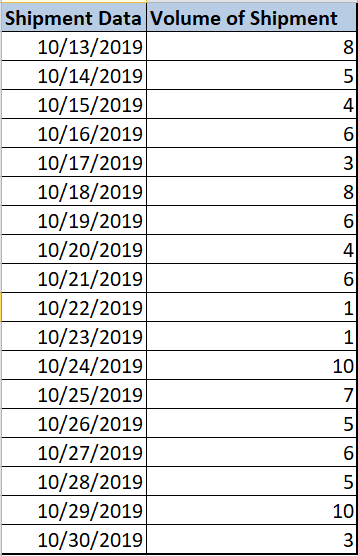
In most real-time cases, we will not be able to collect the entire population data just like hundreds of thousands of observations in our current data. Hence, we depend on the sampling distribution to derive the precise estimates of the population.

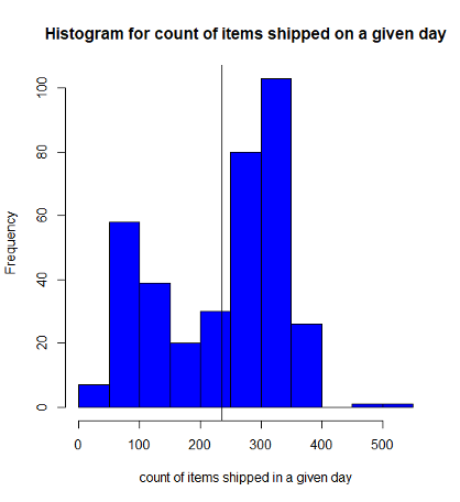
As seen from fig1, the above distribution has a mean of about 236 and a variance of about 102. Looking at this you notice that there is no definite distribution and the spread is way too large. The distribution is nowhere close to a normal distribution. I know it feels sad! Don’t worry. Let’s call CLT to the rescue. This article does not walk you through the proof of CLT, but it illustrates the definition and central limit theorem application.

The Central Limit Theorem states:

“Given a sufficiently large sample size, the sampling distribution of the sample means follows a normal distribution regardless of the population distribution”

I know you are trying to wrap your head around this now! Let me ease this out for you in layman terms: You derive a sample of sufficiently large size from the population and calculate its mean. This is called a sample mean and when you do this for a sufficiently large number of times, you get a large number of sample means. The distribution of these sample means follow a normal distribution regardless of the distribution of the underlying population.

Bear in mind that I apply the central limit theorem only when I do not have population information which is the case in most scenarios but can have sample information and want to derive population parameters such as mean, standard deviation. For your estimate to be very precise, the mean of the sample distribution is more likely to be very close to the population mean.

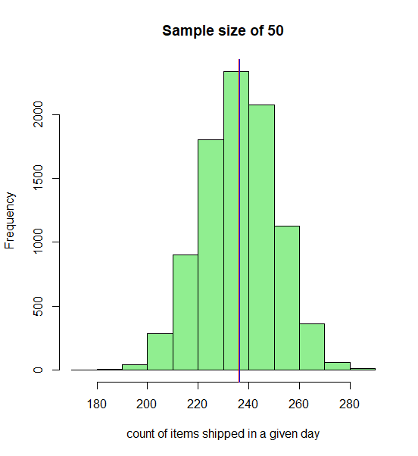
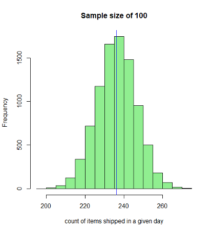
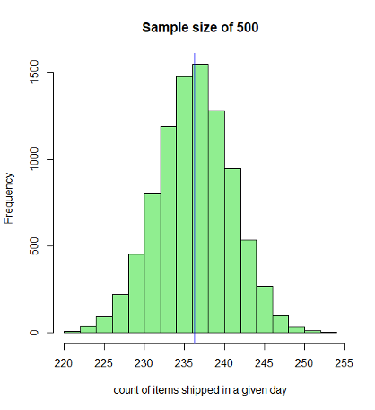
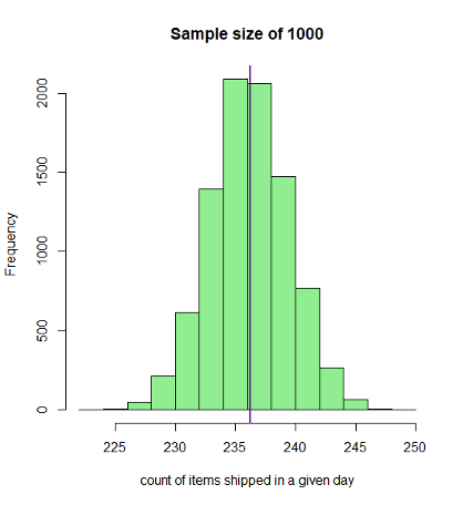
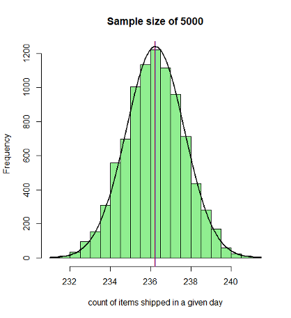
Continuing on this, we will draw multiple independent samples and derive their mean.  As seen from the graphs below, the sampling distribution so obtained approximates to the normal distribution according to the Central Limit Theorem as the sample size increases. When we have a sufficiently larger sample size, say 5000, the distribution approximates very closely to the normal distribution (see below figures).

• 

• 

• 

• 

• 

• 

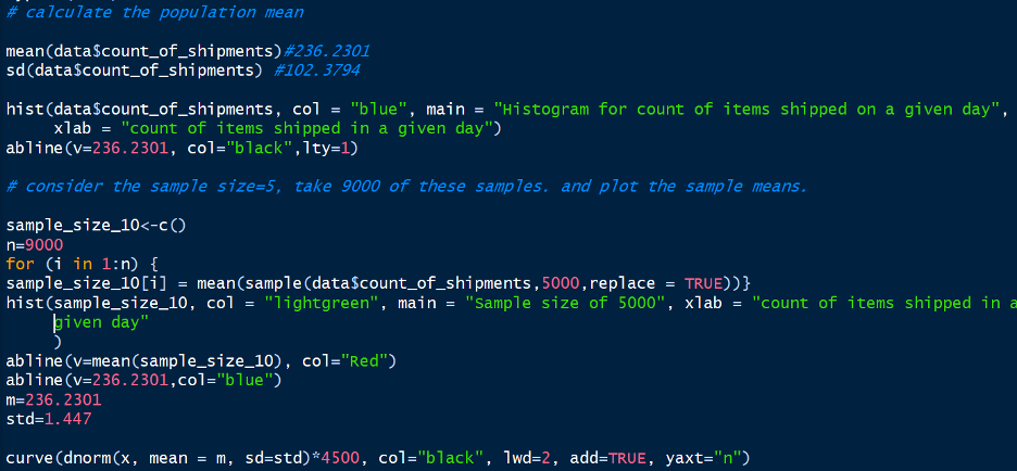
Notice every time I take a sample that is sufficiently greater than the previous ones, the spread becomes tighter thereby increasing the precision of the estimate of the sample. When I plot a histogram and overlay the distribution on it, as the sample size increase, we notice that the sampling distribution becomes more and more normal with almost perfect symmetry around the mean. I have used the R language to plot the graphs. Below is a snippet of the code that I have written to plot these graphs:

This is a very powerful insight that we have derived. When we started we had a random distribution of the population which was nowhere close to normal distribution. With the central limit theorem application, we notice that the sampling distribution (of sufficiently larger sample size, a general thumb rule is 40) approximates to a normal distribution with a mean equal to the population mean and standard deviation of StdDEV.P/sqrt(n) where StdDEV.P is the population variance and n is the sample size. For n=5000, we see a near-perfect normal distribution.

This is an amazing insight that allows us to perform hypothesis testing and derive useful statistical inferences even when your population data is not normally distributed provided you have a sufficiently large sample size.

Let’s Draw Some Inferences

If you closely look at the sample distribution for n=5000, it has elegantly turned into a normal distribution with a standard deviation of about 1.45. The spread around the mean is very narrow indicating more precision of estimates derived. Although I do not have to look at the entire population, I can derive many inferences just by observing the sample distribution, thanks to my dear chap, CLT.

So what questions can we answer about the population by looking at the sample distribution? Well, here are a few of these:

• What is the probability that the shipper will ship more than 300 items per day?
• What is the probability that the number of weekly shipments transacted is 1500?
• What is the 95% confidence interval for the count of daily, weekly, or monthly shipments?
• What is the range for the count of the next set of shipments transacted on a given day? In other words, what is the Prediction interval for the population variable?
• What is the range where most of my shipment counts fall within or say, a range where 90% of my shipment count falls?
• Let’s say the shipper has signed a contract with a new career and would like to see if the mean count of transactions has improved on a daily basis. A hypothesis test could be implemented on the sample to see whether there is any real improvement, say at 95% CI, with the introduction of the new career.

Food For Thought

CLT has a lot of applications in Supply Chain, not only in transportation analytics as we saw above, but also in inventory management. When we consider a single time period inventory model with zero replenishment time, safety stock becomes very significant. For those of you who do not know what safety stock is, it simply means the amount of stock that I keep to meeting my customer’s demand when Inventory on Hand falls below the expected demand. So, the higher the safety stock, the lesser is the probability of stock-outs.

As safety stock is linked to the demand pattern, it is very alluring for the inventory planning community to assume a normal distribution of the daily demand! Although my daily demand is not normally distributed, the demand over N days will surely be normally distributed, thanks to CLT, provided N is sufficiently large and daily demand for N days is independent and identically distributed. Once I have my total demand normally distributed, finding safety stock is a walk in the park!

Wrapping Up

As you can see, the Central Limit Theorem is a very powerful theorem and is helping us to derive a lot of insights. On a closing note, it is very crucial for any supply chain analyst or Logistic engineer or a data science person to be very much aware of the Central Limit theorem to perform validation of the results and to validate the correctness of your estimates.

With a sufficiently larger sample size, you can assume a normal distribution and arrive at more accurate estimates even when your population distribution is nowhere close to a normal distribution. So, now that you have a good grip on the concept of CLT, the next time you chat with your woman, don’t be lame to ask her if she ever wondered what life would be like without the Central Limit Theorem! The situation won’t be “Normal” for sure!

You may also like to read: Basic Statistic Concepts for Data Science