With these fast-paced developments, Machine Learning Models need to be concrete, resilient, and precise. Their prime goal is to make accurate predictions from the given cases, which demands optimization. The core challenge here is to reduce the cost function in Machine Learning algorithms and cope with the potential challenges.
Notably, the cost function improves the model accuracy and lowers the risk of loss by evaluating the smallest possible error. In this article let’s look at what is cost function, different types of cost function, cost function in neural networks, uses, applications, and other properties of cost function.
Also Read: Linear Regression in Machine LearningWhat is Cost Function (CF)?
The cost function also called the loss function , computes the difference or distance between actual output and predicted output.
It determines the performance of a Machine Learning Model using a single real number, known as cost value/model error. This value depicts the average error between the actual and predicted outputs.
On a broader level, the cost function evaluates how accurately the model maps the input and output data relationship . Understanding the consistencies and inconsistencies in the model’s performance for a given dataset is critical. These models work with real-world applications and the slightest error can impact the overall projection and incur losses.
Example
Let us understand the concept of cost function through a domestic robot.
Robots perform superbly in household chores, even for education, entertainment, and therapy. They generally do not require complete human intervention. However, in multistorey homes, they need assistance. This is because domestic robots are ideally programmed to work only on plain floors and are not designed to climb staircases.
Suppose any robot hits the staircase accidentally; it can cause malfunction. Not a complete shutdown but may not function for a short period and then automatically re-start. Like it happens in most robot devices.
With this accidental hit, the robot will eventually note its past action and learn not to interact with the staircases.
It will help the robot to either consider staircases as obstacles and avoid them or may even trigger an alarm.
Overall, the outcome of the incident mentioned above will optimize the domestic robot for better performance. This clearly shows why it is crucial to minimize ML models’ cost function to fine-tune with real-world applications.
Also read: Decision Tree Algorithm in Machine LearningWhy use Cost Function?
Practitioners use the CF in Machine Learning algorithms to find the best optimal solution for the model performance. It is feasible by minimizing the cost value.
With the distance between actual output and predicted output, they easily estimate the extent of wrong predictions by the model. The cost function yields a higher cost value in case of significant discrepancies between the actual and predicted outputs.
The model further undergoes optimization in several iterations to improve the predictions. During every computation, the cost function works as an integral indicator to define the model’s preciseness.
Prominent use cases are cost function in neural networks, linear, and logistic regression.
Optimization method to minimize Cost Function
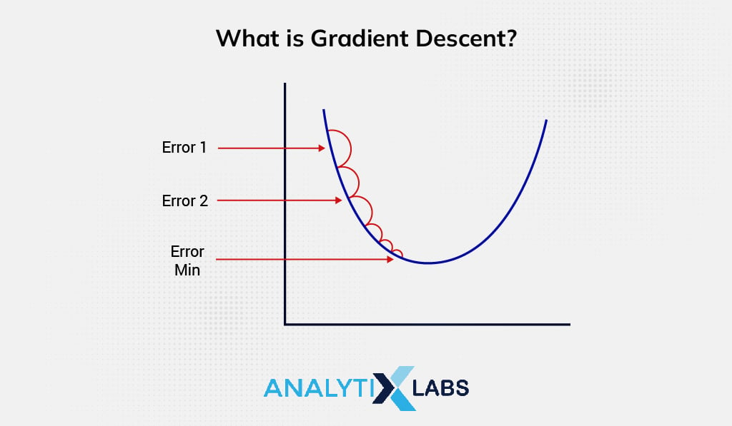
It is possible to have different cost values at distinct positions in a model. Thus, for sustainable utilization of resources (without wastage), immediate steps need to be taken to minimize model errors. Here, Gradient Descent iteratively tweaks the model with optimal coefficients (parameters) that help to downsize the cost function .
The entire approach refers to providing a direction or gradient to the model whereas the lowest point of cost value/model error is known as convergence.
Types of Cost Function
Depending upon the given dataset, use case, problem, and purpose, there are primarily three types of cost functions as follows:
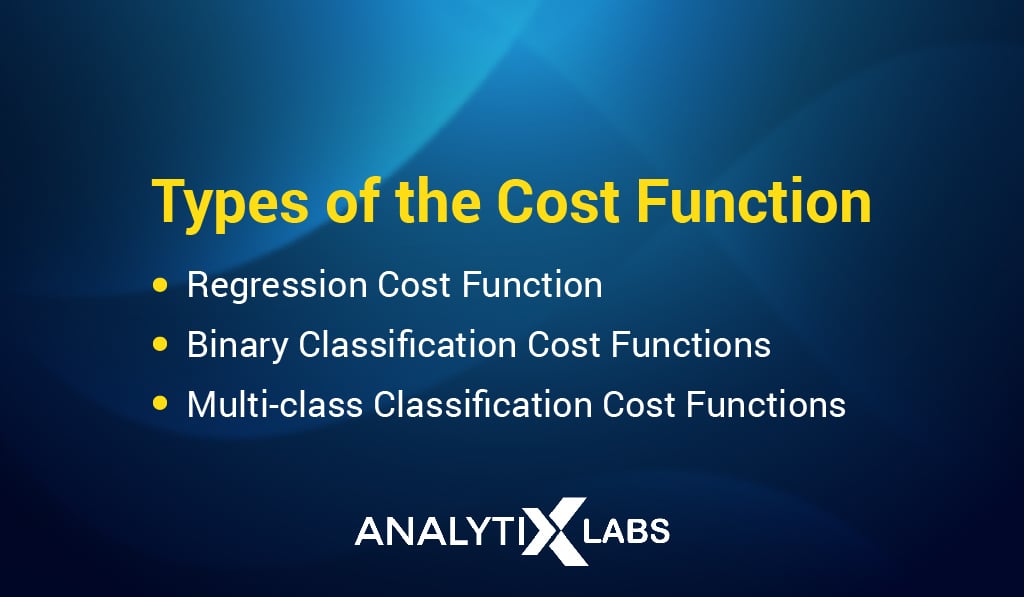
Regression Cost Function
In simpler words, Regression in Machine Learning is the method of retrograding from ambiguous & hard-to-interpret data to a more explicit & meaningful model.
It is a predictive modeling technique to examine the relationship between independent features and dependent outcomes.The Regression models operate on serial data or variables. Therefore, they predict continuous outcomes like weather forecasts, probability of loan approvals, car & home costs, the expected employees’ salary, etc.
When the cost function deals with the problem statement of the Regression Model, it is known as Regression Cost Function. It computes the error as the distance between the actual output and the predicted output.
The Regression Cost Functions are the simplest and fine-tuned for linear progression. The most common among them are:
i. Mean Error (ME)
ME is the most straightforward approach and acts as a foundation for other Regression Cost Functions. It computes the error for every training dataset and calculates the mean of all derived errors.
ME is usually not suggested because the error values are either positive or negative. During mean calculation, they cancel each other and give a zero-mean error outcome.
ii. Mean Absolute Error (MAE)
MAE, also known as L1 Loss, overcomes the drawback of Means Error (ME) mentioned above. It computes the absolute distance between the actual output and predicted output and is insensitive to anomalies. In addition, MAE does not penalize high errors caused by these anomalies.
Overall, it effortlessly operates the dataset with any anomalies and predicts outcomes with better precision.
However, MAE comes with the drawback of being non-differentiable at zero. Thus, fail to perform well in Loss Function Optimization Algorithms that involve differentiation to evaluate optimal coefficients.
iii. Mean Squared Error (MSE)
MSE, also known as L2 Loss, is used most frequently and successfully improves the drawbacks of both ME and MAE. It computes the “square” of the distance between the actual output and predicted output, preventing negative error possibilities.
Due to squaring errors, MSE penalizes high errors caused by the anomalies and is beneficial to Loss Function Optimization Algorithms for evaluating optimal coefficients.
Its more enhanced extensions are Root Mean Squared Error (RMSE) and Root Mean Squared Logarithmic Error (RMSLE).
Unlike MAE, MSE is extensively sensitive to anomalies wherein squaring errors quantify it multiple times (into a larger error).
Binary Classifications of Cost Function
Both Binary and Mutil-class Classification Cost Functions operate on the cross-entropy, which works on the fundamentals of Logistic Regression.
Logistic Regression in Machine Learning purely functions on the probability concept and employs supervised learning algorithms. However, it is pretty complex and utilizes the Sigmoid Cost Function in the predictive analysis algorithm for binary classification problems.
Also Read: Logistic Regression in R (with examples)Binary Classification Cost Functions deal with the problem statement of the Classification Models & predict categorical values like 0 or 1.
It comes under the particular case of categorical cross-entropy, where there is only one probability of output class. Either positive/negative or true/false.
For standard, Class 0 depicts the minimized cost function; the predicted output class is perfectly identical to the actual output. And Class 1 represents the distance between actual output and predicted output.
Multi-class Classification Cost Functions
Multi-class Classification Cost Functions work for more than two classes in the classification model. The functionality is the same as that of the Binary Classification Cost Functions, but with slight extensions.
For standard, here also, Class 0 represents the minimized cost function. But the model error is estimated from higher class score values like it can be 1, 2, 3, etc.
These score values outline the average difference between the actual and predicted probability distributions.
Further, these cost functions utilize the Softmax Function to calculate the probability of an observation belonging to a predicted class . The best real-world application of it is the Cost Function in Neural Networks.
On the whole, the primitive goal of all types of cost functions is to resolve the confusion matrix and foster optimal prediction and flawless functioning in Business Intelligence.
Also read: Breaking the barriers of BI with Data AnalyticsWhat is Gradient Descent?
In machine learning models, training periods are one of the critical phases to make the model more accurate. To understand how precise a model works, you can just run it across required case scenarios. But to know how wrong the model is, or what are the points that cause more faults in the output, a comparative function is required.
Read more on Gradient Descent Algorithm and its variants.
A cost function is a single real number used to indicate the distance between actual output and predicted output in an ML model. To improve the whole model, when this cost function is optimized through an algorithm to find the minimum possible number of errors in the model, it is called gradient descent.
What is Cost Function for Linear Regression?
Now, linear regression is nothing but a linear representation of dependent and independent variables of a particular model that indicates how they are related to finding the maximum possible accurate output for a given parameter.
As the cost function in machine learning demonstrates the points where the model is under-trained, linear regression is used to optimize the functions till the maximum possible points intersect with the regression line.
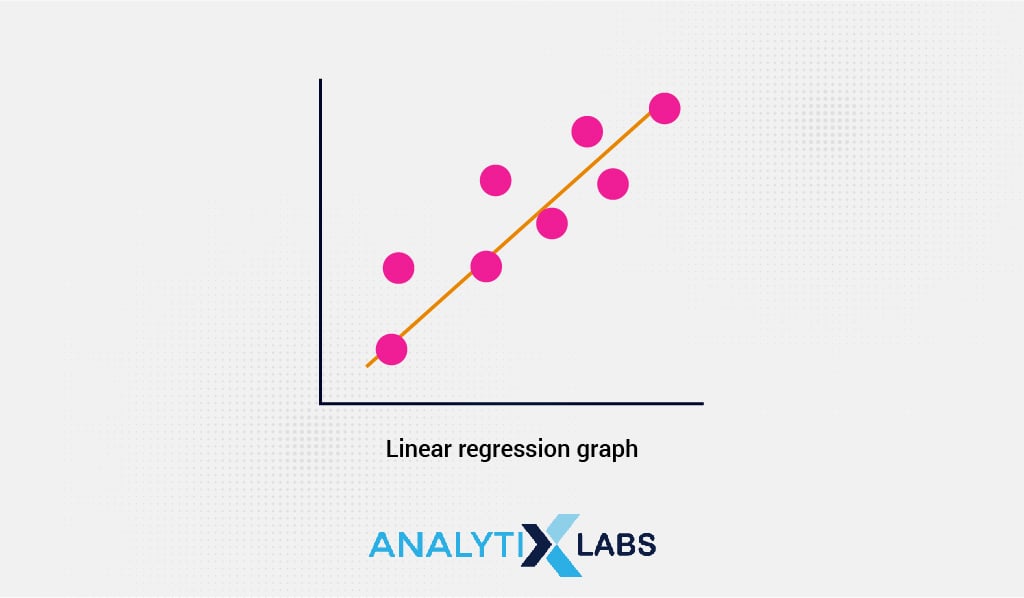
As you can observe from the regression line in this image above, maximum variable points intersect or are near the line, resulting from continuous optimization with respect to the cost function (J).
To improve the machine learning model, we can summarize three key steps as;
- Find the cost function (J) for the respective model to find how much wrong or undertrained the model is.
- Then, to find gradient descent, you need to calculate the small changes in the errors by differentiating the value of J. As there’ll be multiple steps required to make the errors minimized, this step will be performed as a continuous learning approach for the ML model.
- The next step is to plot the linear regression graph to find the point where the error is minimum. It will gradually make the model optimized and efficient.
What is Cost Function for Neural Networks?
An artificial neural network is prompted to work like human brains, learn from mistakes, and improve. As discussed earlier, the cost function is used to find the flaws in an ML model, there is no surprise that neural network is related to this.
There are multiple layers in a real-life machine learning model and neural network algorithms help to find all the errors against different outputs to find the total error. In any neural network, there are different nodes, weights (parameters), biases, and connections. It may seem really complex, but, we can conduct such complex mathematical calculations easily by using technology.
Also read: Understanding Perceptron: The founding element of Neural NetworksHow to find Cost Function of Neural Networks?
- First, you need to calculate the gradient descent as discussed in the earlier section. While the cost function output is decided by the value of the difference between predicted and actual results, gradient descent will replicate the trend of errors.
- According to the slope of the gradient descent, the weight and bias of the neurons will shift in the graph as well.
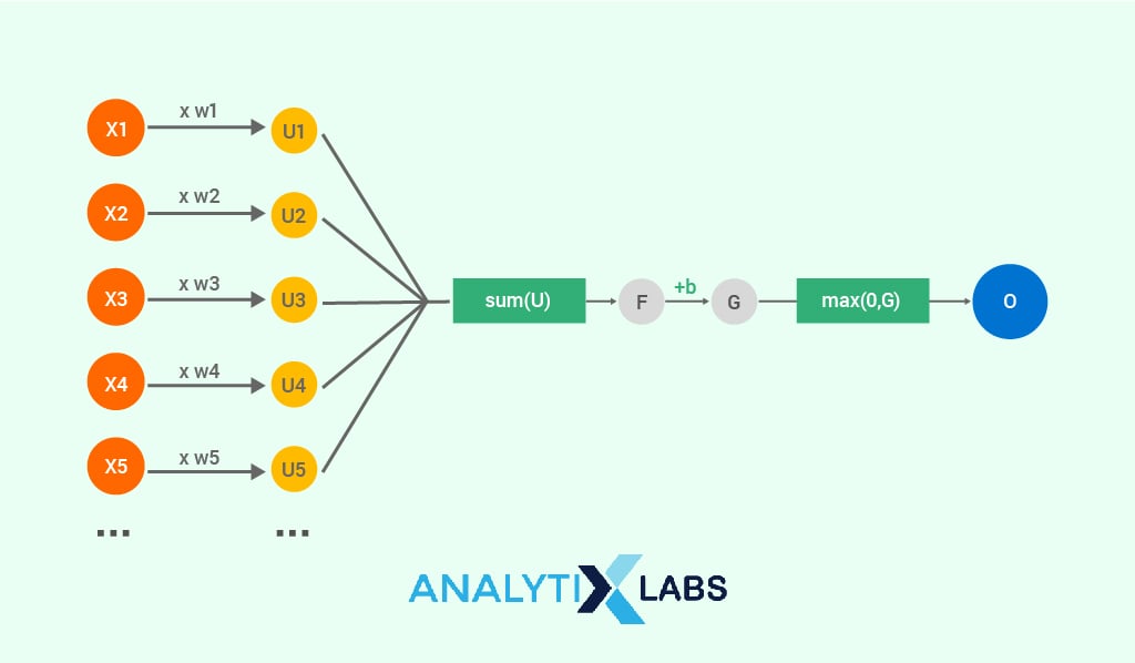
- Then as shown in the image, bias is added with the total error computed from different inputs and intermediate values. This will produce a ReLu value that works as a rectifier for converting any negative values to 0.
Now, it might seem scary to calculate so many complex parameters with accuracy.
Not to worry as Python has all the savior libraries to compute cost functions and find corresponding gradient descent.
How to Implement CF in Python?
Numpy is a Python library that includes high-level mathematical functions to compute on large arrays and matrices. You need to import the ‘NumPy’ and ‘matplotlib’ libraries followed by uploading the dataset. In Numpy, the x-coordinate denotes the inputs and the y-coordinate denotes the corresponding outputs.
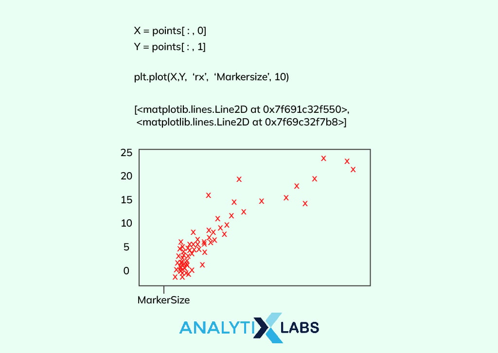
The next step is to set the theta (θ) value in order to predict the x-values. As this is a machine learning model, we also need to set the learning parameters.
We can use user-defined variables like ‘learning_rate’, ‘iteration’, and store the length of points in a variable ‘m’.
To find the cost function value and update the theta value, we need to use operations from the ‘NumPy’ library and the whole calculation will be done in just one line.
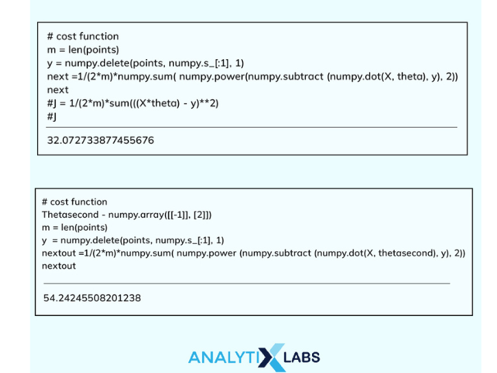
Now, you need to find the gradient descent and print θ for each iteration of the program.
Finally, to plot the graph, you need to use plt.xlabel(‘iterations’) and plt.ylabel(‘J(theta)’) in order to get the iterations in the x-coordinate and corresponding θ values in the y-coordinate of the gradient descent graph .
FAQs:
1. What is Cost Function Formula?
The cost function is a mathematical formula to estimate the total production cost for producing a certain number of units.
Its most common form of the equation is C(x) =FC + Vx where,
- x – no. of units under production
- V – variable cost per unit
- FC – fixed cost
- C(x) – total production cost of a given number (x) of units
The cost function formula also contributes toward evaluating average and marginal production costs.
Businesses use this formula to understand the incurred finances in the ongoing operational period. It helps them monitor profit and loss. The calculation aids in effective decision-making, budgeting, and devising future projections.
2. What is cost function and its types?
The cost function quantifies the relationship between the cost used for production and the output delivered (products/services). It works on an uncomplicated and easy-to-understand mathematical equation.
The cost function graphically represents how the production changes impact the total production cost at different output levels.
Different types are-
- Linear Cost Function in which the exponent of quantity is 1. It works for cost structures with constant marginal cost.
- Quadratic Cost Function in which the exponent of quantity is 2. The average variable cost is represented by a U-shape.
- Cubic Cost Function is represented by a U-shaped marginal cost curve.
3. What is the cost function in economics?
The cost function in economics explicitly defines the financial potential of the business firms. It is fundamentally the inverse proportion of the production cost with the output delivered.
Businesses utilize the cost function to cut down production costs and amplify economic efficiency. Considering the market expenses and cost function projections, they can decide the short and long-term capital investments.
It is pivotal in business planning for achieving optimal production and formulating budget processes. The prime goal is to save costs through efficient resource allocation for profit maximization.
Fundamental Concepts of Neural Networks and Deep Learning
How Data Reduction can increase data mining efficiency?
What is Clustering in Machine Learning: Types and Methods
Artificial Intelligence Engineering: Definition and Applications
How does data compression technique help in data representation?

