Logistic Regression is an algorithm that works in a supervised learning setup where it solves binary classification problems. Learn about the types, purpose, and how logistic regression functions with examples and use cases.
Predictive modeling is an important aspect of Data Analytics and Data Science. While numerous business problems exist, classification is the most common type of problem. Typically, a predictive model must be created to predict classes when solving a classification problem. Numerous algorithms can perform classification, such as Support Vector Machines, Decision Trees, Naïve Bayes, etc. Of the many algorithms, the most fundamental, commonly used, and important algorithm is Logistic Regression. In this article, you will learn what Logistic Regression is and how it functions.
Other article in the Regression Series:
- Learning Logistic Regression: Practical Application in Python [Part 2]
- Logistic Regression in R (with examples)
- Random Forest Regression for Predictive Analysis
What is Logistic Regression?
Logistic Regression is an algorithm that works in a supervised learning setup where it solves binary classification problems.
A supervised learning setup estimates a dependent variable (target) using one or more independent variables (predictors). When the dependent variable is categorical, the problem is known as classification.
There can be many types of classification. One kind is binomial/binary classification, where the dependent variable has two unique classes, typically denoted by 1 and 0.
Logistic Regression is one such algorithm used for resolving binary classification problems.

Logistic Regression outputs probabilities (p) where p defines the likelihood of an observation belonging to class 1.
These predicted probabilities are then converted into classes using a threshold. If the probability is above the threshold, the assumed predicted class label is 1; otherwise, it is 0.
Also read: Sampling Techniques in Statistics [with Probability Sampling Methods]
To fully understand Logistic Regression, you must understand various aspects of this magnificent algorithm. Let’s start with exploring all the major aspects.
Variable Requirements
You must have a basic idea of the type of variables out there to understand the variable requirements of Logistic Regression.
- Binary/binomial
- Continuous
- Discrete
Also read: Types of Distribution in Statistics
| Binary/binomial | A variable is binary when there are only two mutually exclusive values in a variable.
They are typically represented by 1 and 0. In cases where categories are like Yes/No or True/False (binary), Yes/True is usually represented by 1. In the binomial case (where you have two classes that may not be yes/no, such as type of house – ‘rented’/’ own’), 1 is assigned to the class you are interested in predicting. |
| Continuous | A continuous variable can take any numerical value. It can be of type interval where the interval between every two values is equally split (such as temperature in Celsius), or it can be of type ratio with a true zero indicating the absence of a value (such as weight in Kgs). |
| Discrete | Discrete takes any numerical data within a range. Here, the numbers are typically whole or integers.
Discrete can be of two types:
Ordinal is where the numbers have a certain order to them (such as danger level on a scale of 1-5), while Nominal is where there is no order (such as race of individuals denoted by 1=caucassian, 2=Asian, 3=Hispanic, and so on). |
In contrast, ordinal categorical variables are converted to ordinal discrete data. Therefore, all in all, you are always dealing with these three kinds of variables.
The dependent variable must be binary with values 1 and 0 for a binary Logistic Regression to work. In contrast, the independent variable can be a continuous interval, continuous ratio, discrete ordinal, discrete nominal, or binary.
Types of Logistic Regression
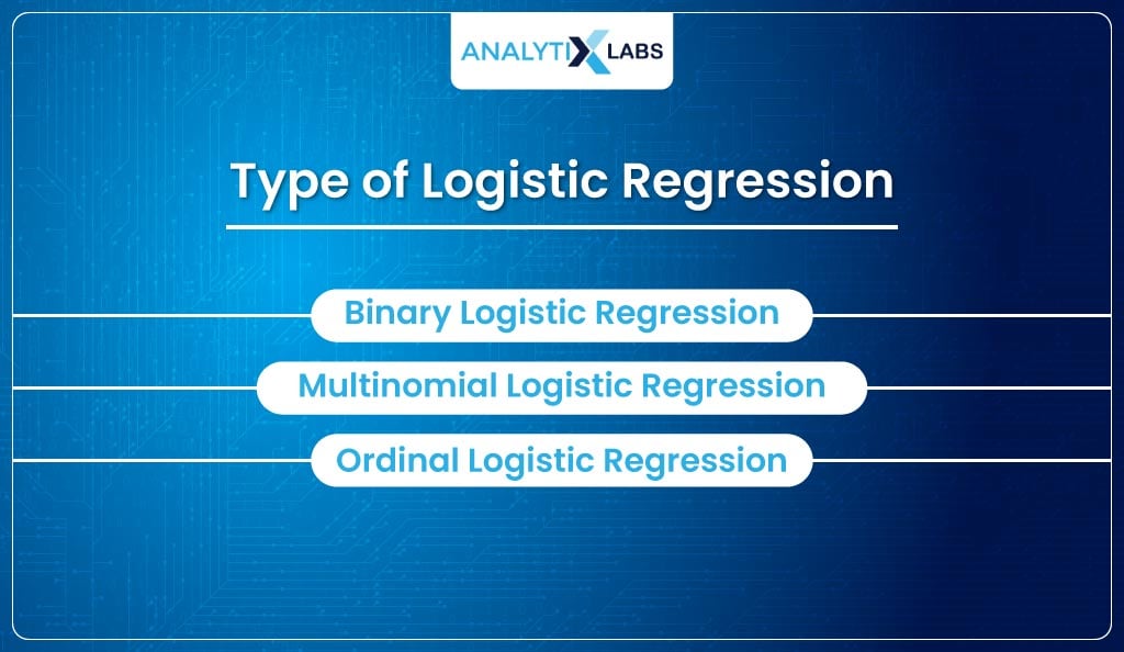
Interestingly, there are many types of Logistic Regression algorithms.
-
Binary logistic regression
This is the most common Logistic Regression algorithm and is the one explored in detail in this article. Here, the dependent variable is binary (e.g., Yes/No, True/False, Sick/Healthy, etc., all denoted by 1/0). This type is so common that when someone talks about Logistic Regression, they usually refer to binary logistic regression.
-
Multinomial logistic regression
It’s another type of Logistic Regression where the dependent variable is a nominal discrete variable. For example, a dependent variable has different types of vehicles like buses, trains, and bikes.
-
Ordinal logistic regression
Lastly, when the dependent variable is an ordinal discrete variable, you use an ordinal logistic regression—for example, when predicting danger levels – Low, Medium, and High.
The most fundamental type of Logistic Regression is binary Logistic Regression, while the other types are just different ways of implementing Binary Logistic Regression only.
Purpose of logistic regression

Another important thing to know is why Logistic Regression is used so prominently.
-
Predict the effects of specific changes.
Logistic regression is a highly interpretable algorithm. It produces coefficients that help you asses how the predictors affect the target. So, for example, if you want to know how much salary to increase to reduce the churn of employees, you can do that using logistic Regression.
-
Predict values
As Logistic Regression helps create a predictive model, it can be used for predicting classes using a given set of predictors.
-
Determine the strength of predictors.
Logistic regression produces a p-value for each predictor that can determine the level of impact it has on the target. For example, using Logistic Regression, you can identify the features that are and aren’t contributing to employee churn.
Assumptions

Logistic Regression is a statistical algorithm, and just like any other statistical algorithm, it has a bunch of assumptions that need to be fulfilled for it to work properly.
| Dichotomous dependent variable | The dependent variable needs to have two classes. |
| No multicollinearity | The independent features should not be related; i.e., they should be truly independent. If there is a high correlation among the independent features, then the Logistic Regression algorithm doesn’t work properly. |
| Relationship of independent variable with log odds | The Linear Regression algorithm requires the independent and dependent variable to have a high correlation; something similar is required in Logistic Regression. Here, each independent variable should have a linear relationship with the log odds (what log odds are is something discussed ahead). |
| Sample Size | Logistic Regression works best with a large sample size, i.e., the number of observations should be high (typically, a value above 300 is considered good). |
| No extreme outliers | Just like Linear Regression, Logistic Regression also gives bad results if there are outliers in the independent variables. |
Properties
Let’s familiarize you now with certain important logistic Regression properties, such as-
- The dependent variable obeys the Bernoulli distribution in logistic regression. The link function links the predictors to the target’s Bernoulli distribution having unknown probability ‘p’.
- Predictions, i.e., the probabilities, are based on the maximum likelihood.
- Logistic Regression has fundamentally different ways of evaluating model fitness. For example, the AUC score is used instead of the coefficient of determination(R-squared) in Linear Regression.
Equation
The next important thing you must know is that Logistic Regression is a member of the Generalized Linear Models (GLM). Generalized Linear Models aim to establish a linear relationship between the predictors and the target variable to produce predictions.
The most common linear algorithm is Linear Regression, which fits a straight line to predict the real values using the equation-
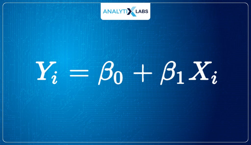
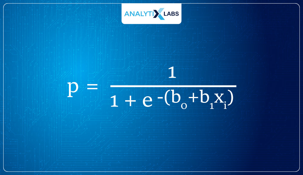
Logistic Regression, on the other hand, uses a link function known as logit to map the relationship between the target and the predictors. As the aim is to predict probabilities, the logit function is transformed to return probabilities.
This modified logit function, known as the sigmoid function, fits an S-shaped curve to the data that produces probabilities for class 1 using the equation –
Key Terminologies and Concepts
Next up, you need to be aware of some basic concepts that will help you in the discussion on how Logistic Regression works. These key terminologies will be discussed in detail in the subsequent sections.
-
Logistic function
It is a function that represents the relationship between the dependent and independent variables. It transforms the input probability, indicating the likelihood of the dependent variable being of class 1.
The logistic function is the sigmoid function.
-
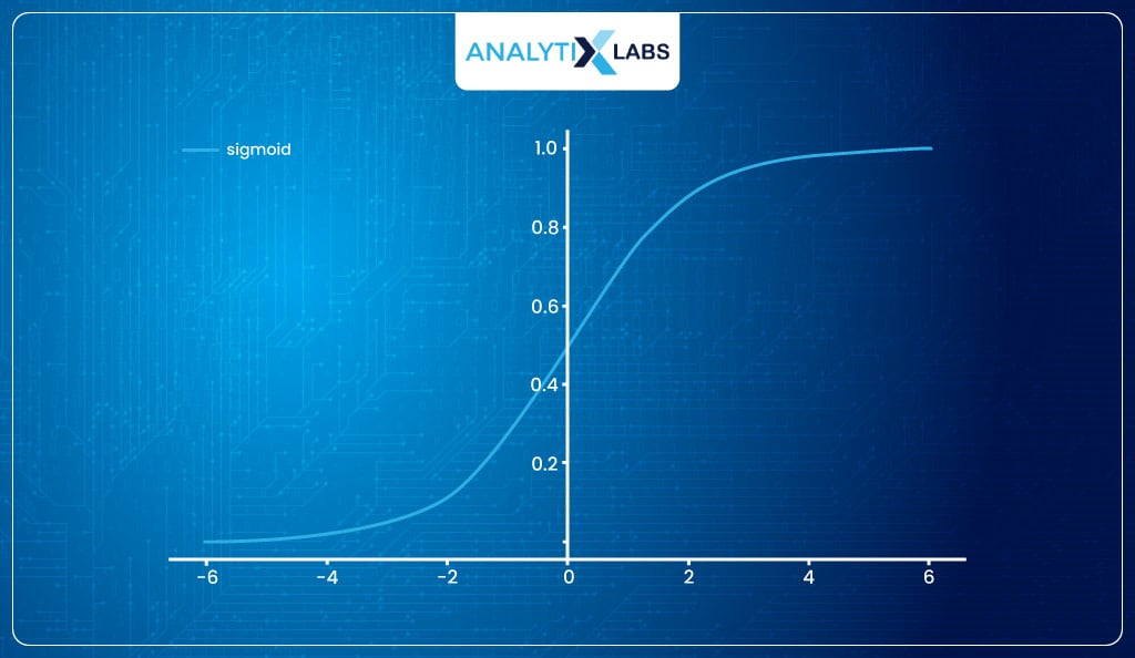
Sigmoid function
It is a function that can map any real-valued number into a value between 0 and 1. It produces an S-shaped curve.
-
Coefficients
They are the parameters in the Logistic Regression responsible for explaining how the independent variable is related to the dependent variable.
-
Bernoulli trial
It is an experiment that has two outcomes. For example, a coin toss is a Bernoulli trial as it will have heads or tails as the output.
-
Bernoulli distribution
It is a discrete distribution of a Bernoulli trial. So, for example, for a coin toss where the probability of getting heads or tails is 50-50, the Bernoulli distribution will look like-

-
Binomial distribution
The Bernoulli distribution is where the number of trials = 1. The binomial distribution is the Bernoulli distribution with the number of trials> 1.
For example, if you repeatedly toss a coin and plot the outcomes, you will get a binomial distribution.
-
Probability
Probability is the ratio of a particular event happening to all possible events that can happen. It’s calculated by dividing the number of trials where you noted an event (or outcome of interest) by the total number of trials.
For example, 100 football matches (trials) took place between Manchester United (MU) and other teams where MU won in 25 matches (event/outcome of interest). Therefore, for the next match, the probability of MU winning is 25/100 = 0.25, i.e., 25%.

-
Odds
Odds refer to the ratio of the probability of the event happening and the probability of the event not happening.

Using the previous example, the odds of MU winning will be
- Probability of MU winning / Probability of MU not winning
= 0.25/0.75
= 0.33
Thus, the odds of MU winning is 0.33, i.e., 1 win to 3 losses or, as commonly said, 1 in 3 chance of winning or, in other words, roughly one-third likely to win a match.
-
Odds ratio
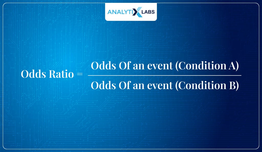
The odds Ratio (OR) is the ratio of two odds obtained from two different conditions.
For example,
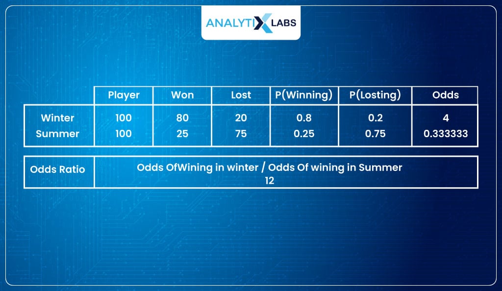
- In the winter season, of the 100 matches played, they won 80 matches, providing us with the odds of winning as 80/20 = 4
- In the summer season of the 100 matches played by MU, they won 25 matches, providing us with the odds of winning 25/75 = 0.33
- Now we can calculate the odds ratio that will be:
= 4/0.33
= 12
This means that MU is 12 times more likely to win when playing in the winter.
You interpret the odds ratio such that.
- If OR > 1 🡪 , the numerator is greater than the denominator. Therefore, the odds of the event happening are higher for the conditions mentioned in the numerator.
- If OR < 1 🡪 , the numerator is lesser than the denominator. Therefore, the odds of the event happening are lower for the conditions mentioned in the numerator.
- IF OR = 0 🡪 Odds of an event occurring are the same in both the conditions
If, for example, the odds had been the same because they won only 25 out of 100 matches in both the summer and winter seasons, then the odds ratio would have been 0.33 / 0.33 = 1, meaning that they are equally likely to win when playing in summer or winter conditions.
Knowing all this is important because, in logistic regression, the beta coefficient (β1) of an independent variable (x1) estimates the increase/decrease in the log odds of the interested outcome per unit increase in the value of the independent variable (x1).
The exponent of a beta (e β1) indicates the odds ratio associated with one unit increase in the independent variable.
Advantages and Disadvantages of Logistic Regression
Let’s also discuss a few of the most prominent advantages and disadvantages of the Logistic Regression algorithm.
| Advantages | Disadvantages |
|
|
|
|
|
|
Advantages
The most crucial advantage of Logistic Regression that makes it one of the most used algorithms is that-
- East to implement: It’s easy to work with Logistic Regression as there are not a lot of complicated parameters to tune. It is relatively easy and simple to train a Logistic Regression algorithm.
- Good for linearly separating data: As Logistic Regression belongs to the family of Generalized Linear Models, it can easily solve linear classification problems.
- Provides insights – High on interpretability: Logistic Regression is extremely easy to interpret. It’s possible to understand how it is coming up with the predictions and thereby is not opaque.
One can use the independent features coefficients, standard errors, p-value, etc., to understand how relevant a feature is, how it causes the probabilities to change, etc. This is why wherever in-depth analysis needs to be done, Logistic Regression is used.
Disadvantages
There are, however, some major disadvantages of Logistic Regression that you must keep in mind when using it.
- Fails when the target is continuous: You cannot use this algorithm if the dependent variable is continuous. For that, you have to use other algorithms like Linear Regression.
- The assumption for linearity between dependent and independent variables: Logistic Regression, being a linear classifier, requires the dependent and independent variables to have a linear relationship to perform classification successfully.In reality, however, having such data is difficult to find, making it difficult for Logistic Regression to classify the two classes linearly. Therefore, it fails when trying to solve nonlinear classification problems.
- Inaccurate if the sample size is small: It requires a good amount of data for both classes. Smaller datasets can cause the model to overfit.
As most of the aspects around Logistic Regression have been covered, it’s time to get into the nitty gritty of this algorithm and understand how it works.
How Logistic Regression Works?
Suppose you have a dataset where, in the dependent variable, you have two classes – hatchback and SUV, indicating the type of car. At the same time, the independent (predictor) is the car’s weight.
You want to predict the type of car based on its weight. You, therefore, decide to use Logistic Regression that will return the probability of observation of belonging to class 1 (SUV).
However, to properly understand how Logistic Regression will produce output, you need to understand three concepts –
- Logit function
- Sigmoid function
- Maximum Likelihood Estimation
Logit and Sigmoid Function
At its core, Logistic Regression is like Linear Regression because both are linear models. Both belong to the family of Generalized Linear Models, which linearly map the relationship between dependent and independent variables.
The Logistic Regression model, however, uses a specific function known as a link function to squeeze (or convert) the output of Linear Regression between 0 and 1 so that it can indicate probabilities.
This ‘specific’ link function in the case of Logistic Regression is known as the ‘logit’ function .
Let’s understand this logit function.
Fitting Linear Equation
In Linear Regression, the equation for the line of best fit is-

A common question that gets thrown around a lot is the difference between linear and logistic regression, or why can’t we use Linear Regression to solve a binary classification problem?
The answers to all these questions can be found by trying to fit the Linear Regression equation and solving a binary classification problem.
- The problem with the above equation is that it predicts continuous values and is used when the target variable is continuous. On the other hand, we require it to predict probabilities (y). Therefore, we rewrite the equation such that-
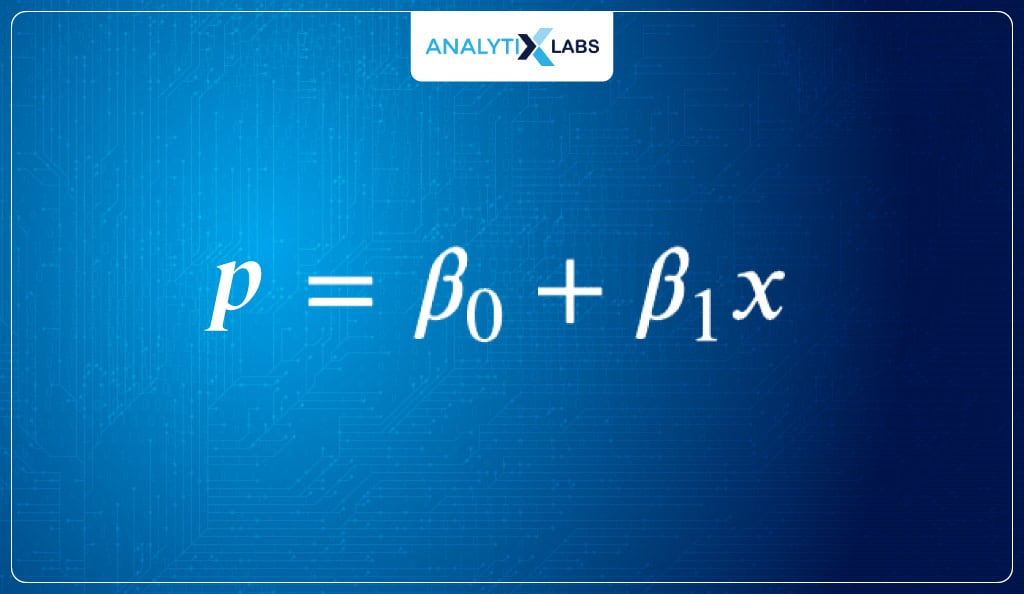
- The output is P, i.e., probabilities; therefore, the equation aims to predict probabilities. The output can go below 0 or above 1 using the above equation to predict probabilities because β0 + β1x1 will generate a linear line.
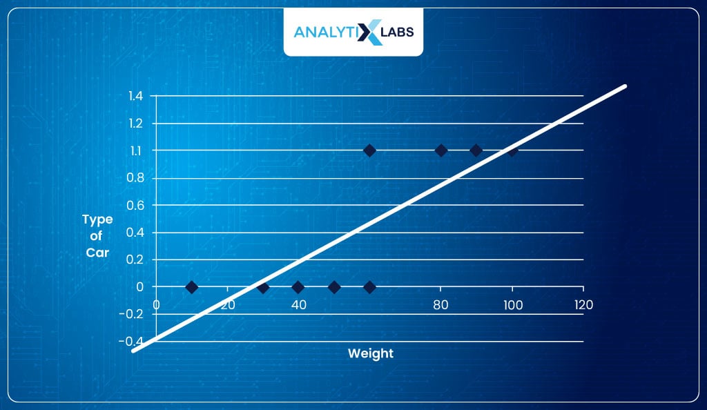
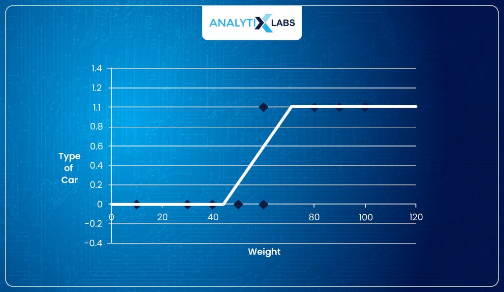
As you know, the probabilities are always in the range of [0,1]. Therefore, rather than fitting a straight line, we need to fit something like this-
Introducing Odds
The shape of the line looks like an ‘S’. Therefore, we need an S-shaped curve to fit the data. If we manage to get one, the output will indicate the probability of an observation belonging to class ‘1’ such that the higher the output, the more probable the observation belongs to class 1.
Fortunately for us, there is a function that returns such a curve.
It is known as the sigmoid function. The way equation for a straight line is y = β0 + β1x1; the equation for the sigmoid curve is 1/1+e-(β0+ β1×1). The question, however, is how to move from the current equation to the sigmoid curve.

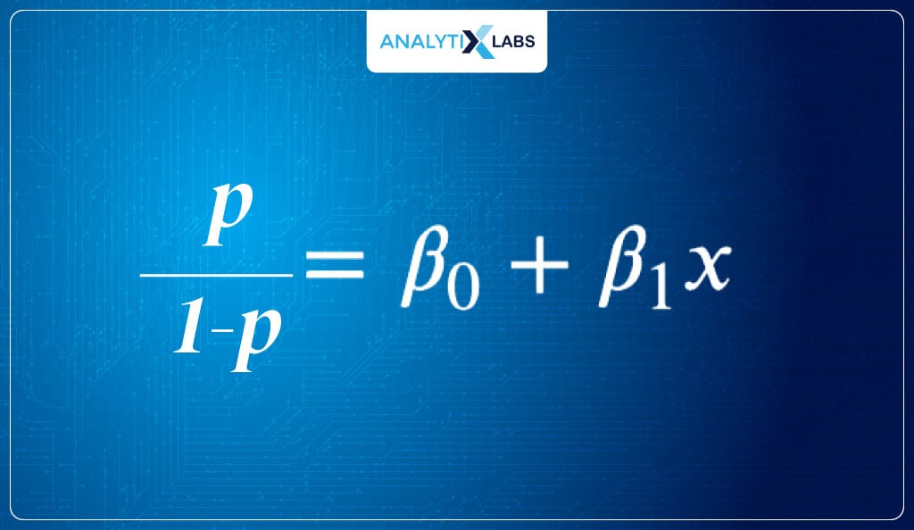
Let’s start moving towards an equation that returns probabilities with a range between [0,1]. The problem we have is that the current function can return negative output. We overcome this issue by taking the odds of P.
Introducing Log Odds
So far, so good. But the problems are not solved yet. While the good thing is that the odds cannot be negative, the problem is that they don’t have an upper limit, i.e., they can go to infinity.
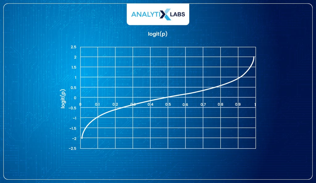
Therefore, the above equation’s output range is [0, +∞]. This is where things will get interesting. I now take the log of the target, i.e., I consider the log of odds.

This gives me a logit function, the link function in our case.
logit (P) = log(odds) = log (P/1-P)
Taking the inverse of log odds (logit)
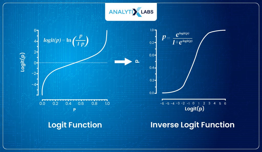
The logit function returns values with a range of [-∞, +∞]. But this is where you will understand why we use the logit function.
The logit function maps the probabilities (having range [0,1]) to real numbers (having range [- ∞,+ ∞]), but the great part about it is that if we take the inverse of the logit function, we get a function that maps the interval [- ∞,+ ∞] monotonically onto the probabilities [0,1].
Thus, the inverse logit function will generate values between [0,1]. The inverse of logit is –
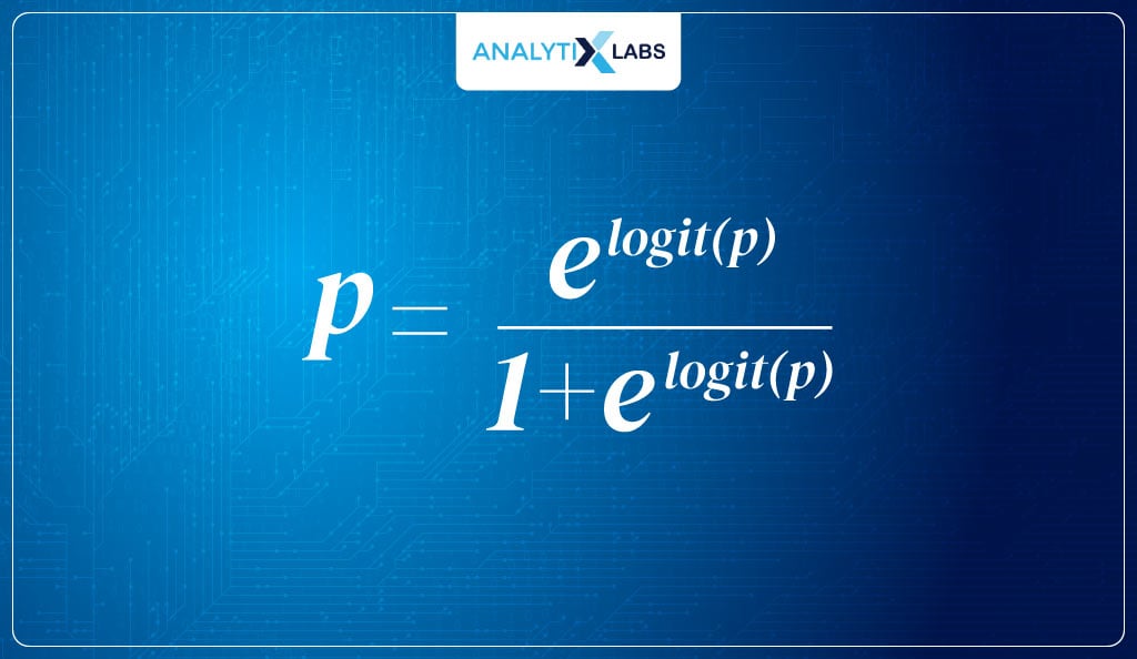
Therefore, we used the logit function to calculate its inverse and find the sigmoid curve that can return the probability of an event occurring.
Deriving Inverse Logit from Logit
The question that you might be having is how you move from the logit function to the inverse logit function, i.e.,
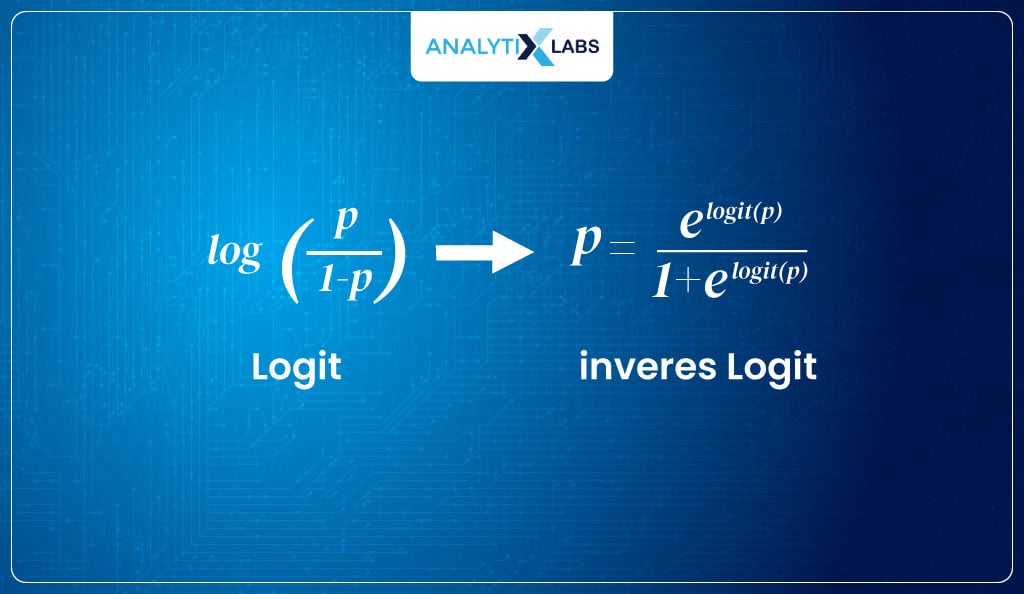
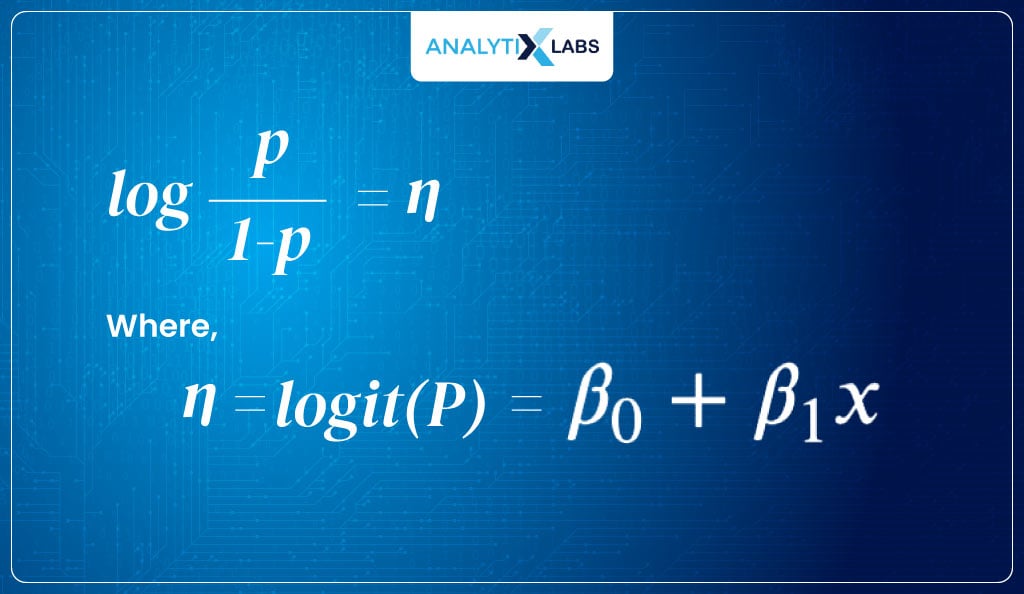
- To get to the inverse logit, we take the above logit equation where we are using the log odds of the probability and multiply both sizes by the exponent and get the following:
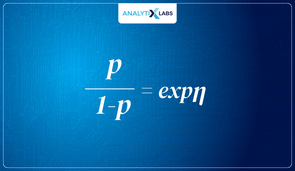
- We then solve for P such that we first multiply 1-P from both sides, giving us:
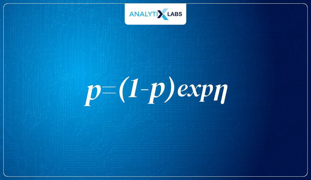
- Now we multiple (1-p) with expn providing me with:

- Next, we add p*expn to both sides, giving us-
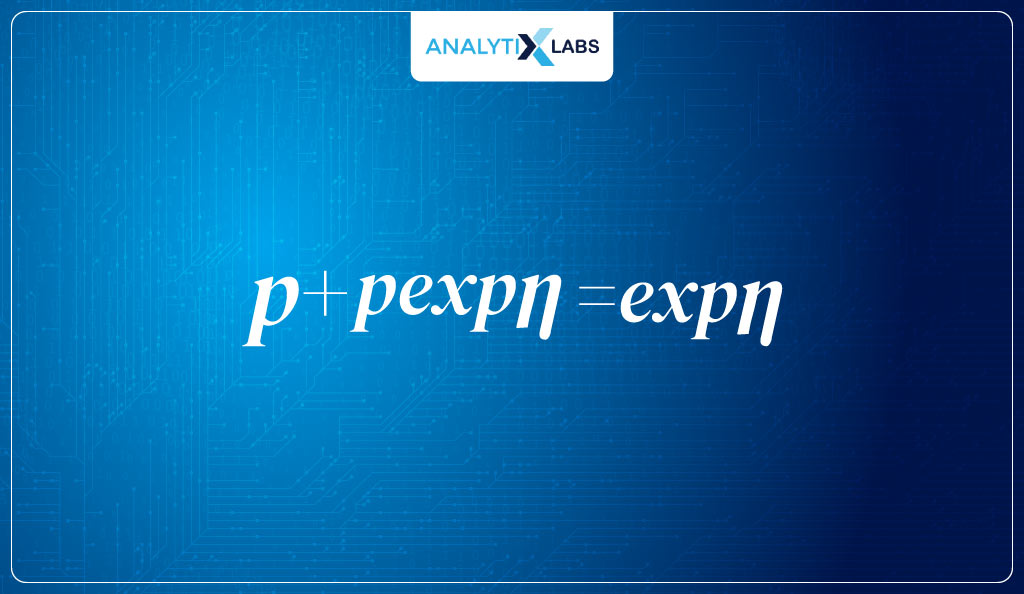
- Now we pull p out of the left side of the equation, leaving us with-
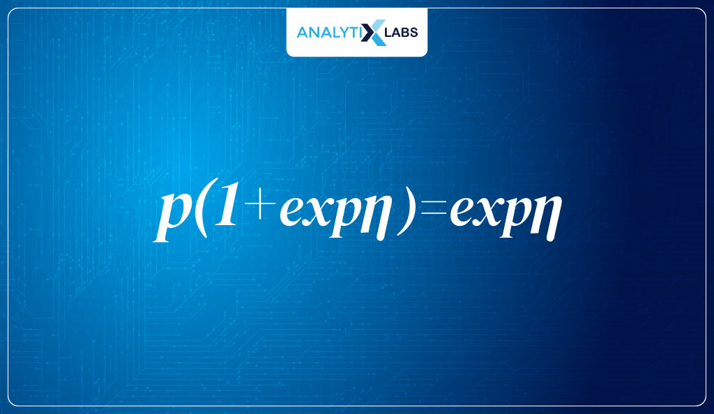
- Lastly, we divide both sides by 1+en to get the inverse logit

Logistic Function – Sigmoid
As discussed earlier, the sigmoid function is:

It is very similar to the inverse logit function. It’s because the sigmoid function is nothing but the inverse logit function. By dividing the numerator and denominator of the inverse logit function by e(b0+b1x), you can get the required sigmoid function, aka—the estimated regression equation, aka—the logistic function.
Maximum Likelihood Function
The next thing we can do is estimate the parameters. Here, the primary parameter for us is the betas.
Cost Function of Linear Regression
Now, let’s step back and recap how a Linear Regression works. In Linear Regression, a linear equation comes up with the predictions (ŷ ). The linear equation is β0+ β1x1, where the value of β1 and β0 dictates the slope and intercept of the line.
Let’s consider β1, i.e., the slope, for now. For different values of β1, different linear lines can be created.
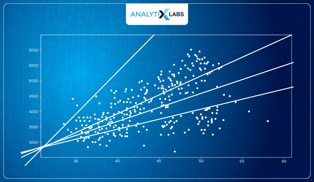
The question is how to find the best line, i.e., the line of best fit. This is where the concept of ordinary least squares (OLS) comes into play.
The process starts with taking random values of the parameters (β0 and β1) and predicting values (ŷ). The error is then calculated, which is (ŷ- y)2, and the sum of all such errors is taken. The parameters are then optimized so that this error is minimized. Therefore, the error, aka the cost function, can be calculated using the following Mean Squared Error (MSE) equation-
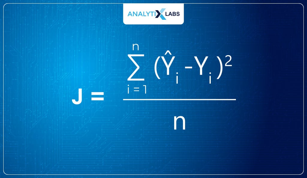
The cost function is always created so that its minimum value is tried to be found (it’s a convention in machine learning to create optimization problems in such a way that a minimum is to be found).
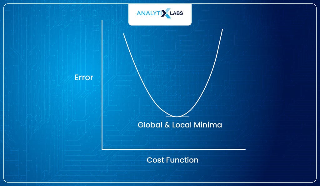
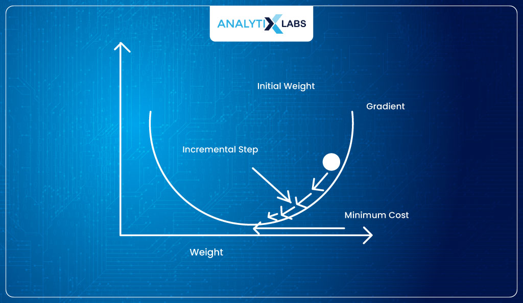
This is where optimization algorithms like gradient descent come into play that use concepts of derivation like the chain rule and other partial derivatives concepts to tune the parameters so that the loss is minimized with each iteration (each iteration is a round of tuning parameters and calculating the error).
Eventually, after repeatedly tuning the parameter, the optimization process stops when it converges, i.e., when no further error reduction occurs.
Need for finding a new cost function in logistic regression
Now, let’s take the cost function of Linear Regression forward and understand it in the context of logistic Regression.
We need to find the value of the parameters (b0 and b1) such that it produces maximum accuracy (or least error). However, we don’t have anything like OLS here where we can calculate the sum of square error by calculating Σ(ŷ- y)2.
This is because, in our case, while the ŷ are probabilities, y contains binary classes. Therefore, we need a different mechanism to find the “sigmoid curve of best fit” (this is where the Maximum Likelihood Estimation (MLE) method will come in handy).

Remember the previous example of car type and weight. Suppose you create a Logistic Regression with four different β values to get the following four sigmoid curves:
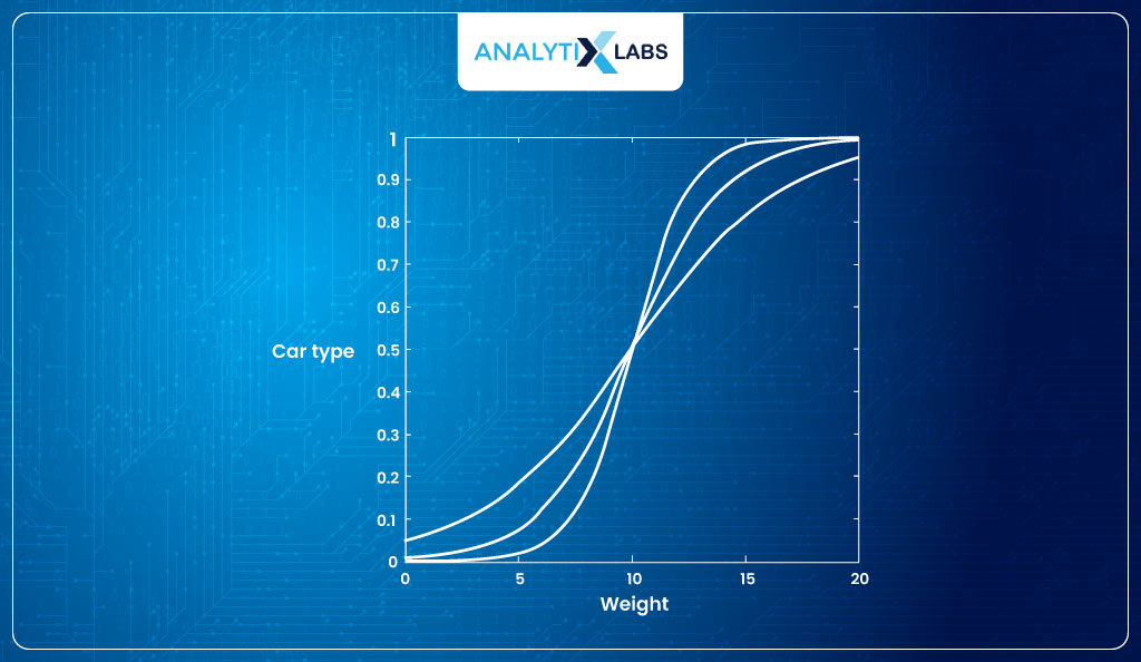
The question is how to identify which sigmoid curve is best for us. Like Linear Regression, we can think of optimizing for the parameters, but what will our cost function be? There will be trouble if we try to use the MSE equation used in Linear Regression.
The function ŷ = 1/1+e-β0 + β1 is a nonlinear function that will cause the cost function to have a non-convex graph with multiple local minima. We will probably converge on the local minima rather than the global minima. Hence, we need a different cost function.
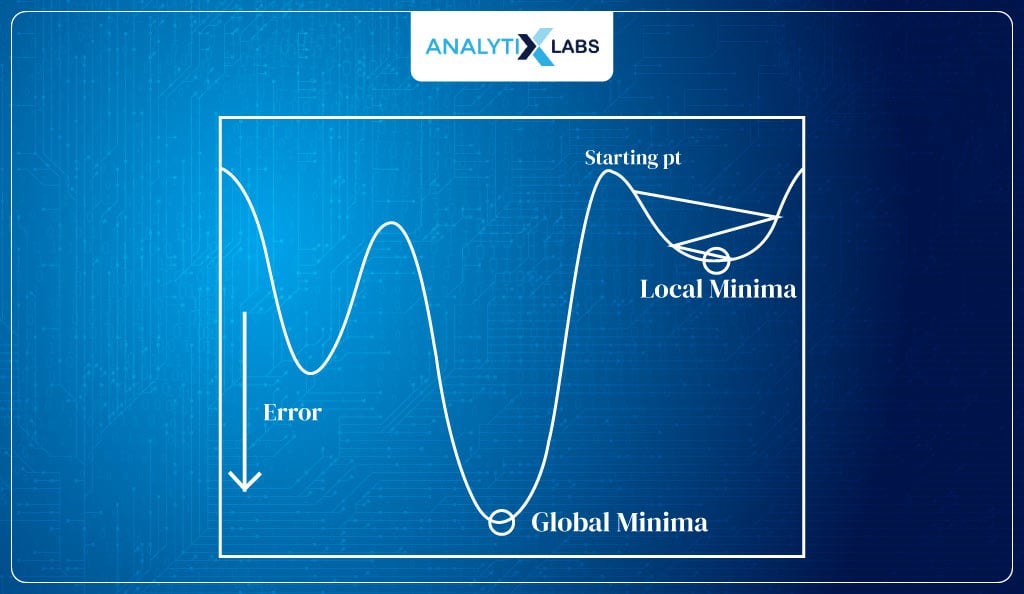
Process of Maximum Likelihood Estimation
The cost function known as the log loss can be used for finding the parameters in Logistic Regression as it will not give us any trouble, unlike with MSE.
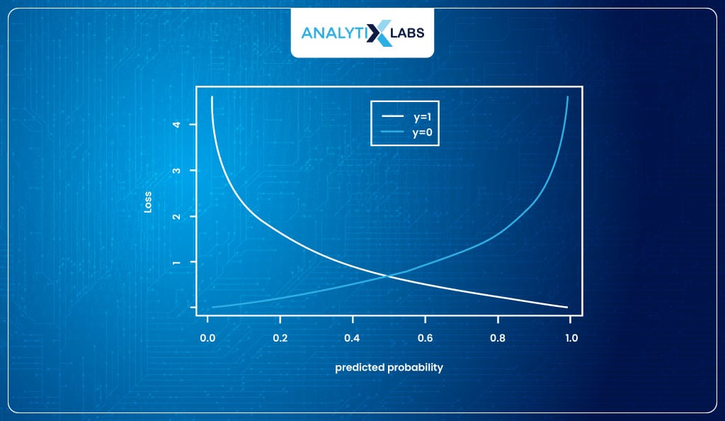
The log loss function is provided to me by the Maximum Likelihood Estimation method, which states that probabilities should be such that it maximizes the chances of producing the correct answer , i.e., maximizes the log-likelihood.
Now, you might wonder how Maximum Likelihood Estimator works to find the log-likelihood. Let’s understand this with an example. Suppose you have the following data-
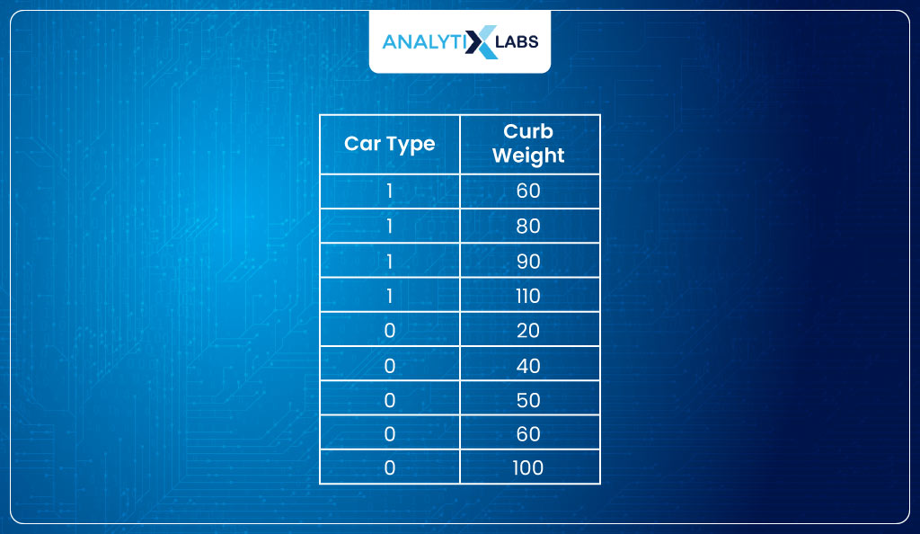
(Hypothetically speaking) the model considers β0=0.02 and β1=0.2, such that the probabilities come out to be:

With the sigmoid curve (again hypothetically speaking) looking something like:

- To understand how good this model is, we calculate the log-likelihood. Likelihood means how close each class’s probability is to the desired value.
- Ideally, the probability of all observations where the label is 1 should be high (equal to 1). Similarly, the probability should be low (equal to 0) for all observations where the class label is 0. I say this because the model predicts probabilities (p) as the likelihood of an observation belonging to class 1.
- In other words, the sum of probabilities belonging to class 1 should be high for all observations where the class label is 1. Similarly, the sum of probabilities belonging to class 0 should be high for all observations where the class label is 0.
- To calculate this, I take the sum of the log of p (probability) where the class label is 1 and the log of 1-p where the class label is 0. This sum is what is referred to as the log-likelihood.
Below is the calculated the log-likelihood:
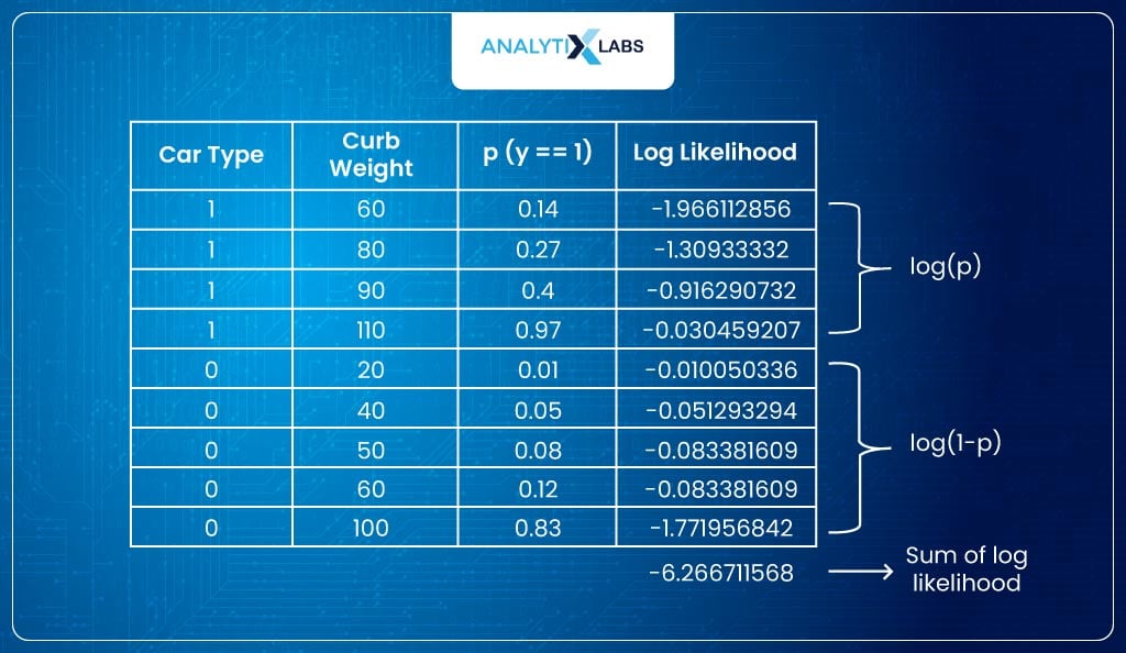
Now (hypothetically speaking), if we create another model but this time using β0=0.05 and β1=0.4 such that the probabilities come out to be:
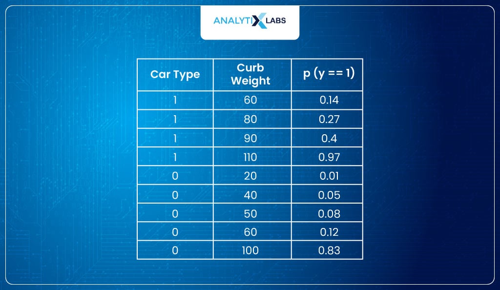
Making the sigmoid function to look like –

If now, for this model, the log-likelihood is calculated, it comes out to be 5.4, which is lower than before.
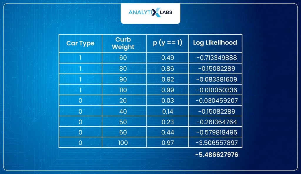
This is because this sigmoid function fits better to the data such that probabilities (y==1) for class label 1 are higher and 0 are lower.
Log Loss
In machine learning, the idea is to tune the parameters to maximize accuracy. Therefore, we have something to tune: this sum of log-likelihood (or “log-likelihood”).
Log Likelihood can, at best, be 0 where the model fits perfectly such that the probability (y==1) is 1 for all observations with class label 1 and 0 for all observations with class label 0.
For models that don’t fit well, the sum of log odds is a large negative number that can go up to infinity. Thus, its range is [-∞, 0] because I am taking logs of values whose range is [0,1].
Log loss by the optimization algorithm is tried to minimize by tuning the β parameters. Therefore, the lower the log loss, the higher the model’s log-likelihood. Thus, the cost function for Logistic Regression (when using MLE for tuning parameters) looks like this-
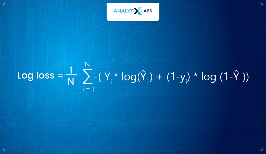
To summarize whatever we have learned in this section, let’s take a dummy dataset and roughly follow the process undertaken by programs that run Logistic Regression for you.
-
Summarizing using Excel
To revise whatever you have learned regarding the working of logistic Regression, let’s build a small Logistic Regression model in Excel.
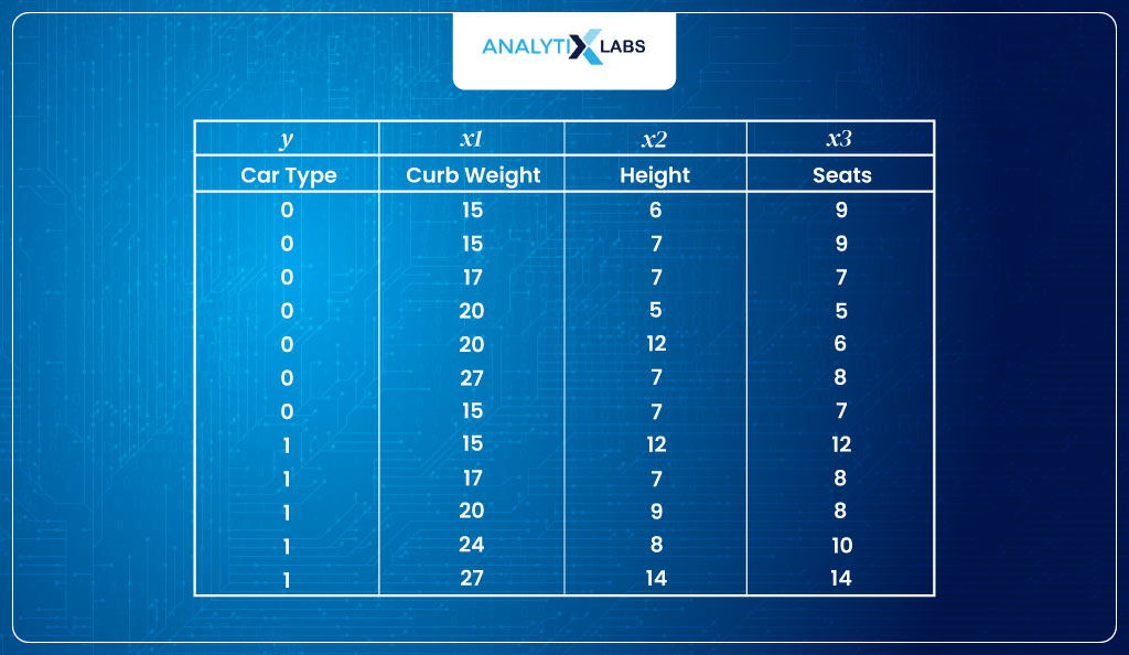
- Input dataSuppose you are dealing with the following dataset with car type as the dependent variable, with 0 indicating hatchback and 1 indicating SUV. There are three predictors – curb weight, height, and the number of seats.
- Initializing processThe first step is to have a logit. As discussed earlier, logit is the log of odds, i.e.
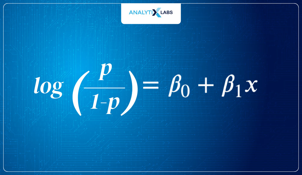
In this example, as there are three predictors, the logit equation will be: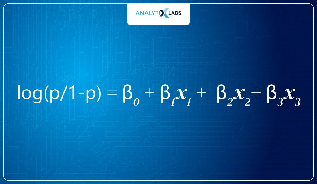
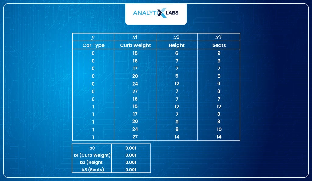
- However, before calculating logit, we need the parameter values, i.e., the β values.We initialize the process by assigning random initial values for all four β values (here, We have assigned a value of 0.001 for all four β)
- Calculate log odds (logit)Next, we use the logit function to calculate the log odds.
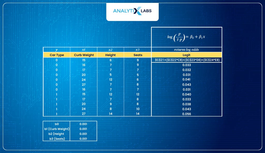
- Calculate probabilities (inverse logit)As discussed, the logit function returns log odds, but the range of these values is [- ∞,- ∞], which we don’t want. Therefore, we use the inverse logit that will return probabilities.
 As you can see below, this is what we have done:
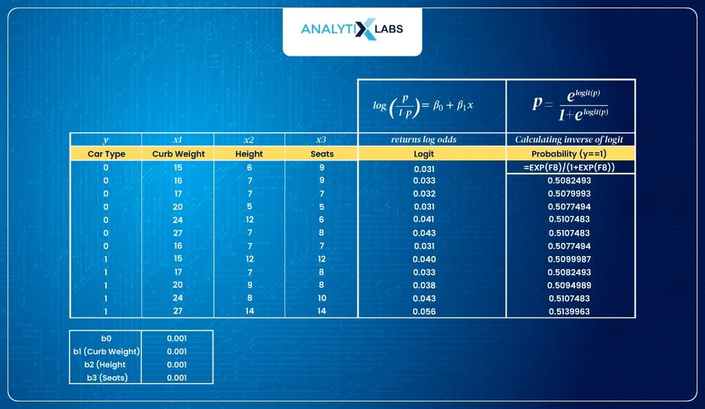
- Calculate log-likelihoodWe calculate the log-likelihood. Here, for the negative labels, we calculate the log-likelihood by taking the log of 1-p (because the predicted probabilities are for label 1, so, to find the probability of an observation of class 0 belonging to class label 0, I perform 1-p).For the observation where the class is 1, we take the log of p. We then sum all these likelihood values to get the sum of the log-likelihood, called log-likelihood.
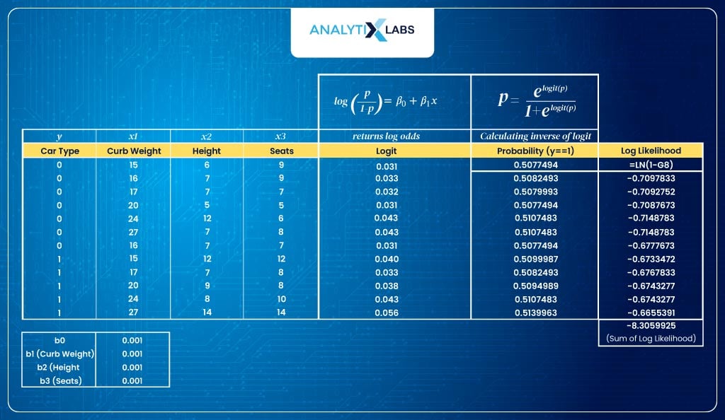
- Optimize the parametersFor the initial values of β, I am getting a log-likelihood of -8. This is where the optimization process starts. We need to find those values of β that maximize my log-likelihood.In sophisticated statistical models, various optimization algorithms like gradient descent are used. Here, we use the solver functionality of Excel.To install Solver in MS Excel, go to File > Options > Add-Ins > Solver > Go. Once done, you will sill the solver function under the Data tab in the Analysis group.To make Excel maximize the log-likelihood by tuning the β values-By performing all these steps, we let Excel try different values of β to maximize the log-likelihood.After solving for the β values, our new log-likelihood is -5.9, higher than the previous -8.3.>> Set the cell calculating the sum of log-likelihood as the objective and setting the objective to max
>> Provide the range of cells having the β values under the ‘By Changing Variable Cells’ option
>> Untick the ‘Make Unconstrained Variables Non-Negative’ (so that my β values can go negative if required)
>> Lastly, choose the solving method as GRG Nonlinear and click Solve To analyze, let’s look at the predicted probability before and after optimizing the threshold. As you will see, for many observations of class 0, the probabilities have been moved closer to 0, whereas, for a few observations of class 1, the probability is now much closer to 1.

Let us now discuss how you will interpret the results gained from a Logistic Regression model.
Interpreting Results
While Linear and Logistic Regression return β values, how you interpret them differs. In logistic Regression, the β value refers to the change in the log odds of an event happening for a unit increase in x.
Let’s take the final equation of the above example to understand how the logistic regression output is to be interpreted.
y = -6.57 + -0.11*weight + 0.40* height + 0.68*seats
Coefficients:
- The β1 (weight), β2 (height), and β3 (seats) explain the change in log odds in the probability.
- So, for example, a β of 0.4 for the feature height means that for every unit increase in height, the log odds of the car being of category 1 (SUV) increase by 0.4.
- Interpreting log odds is a bit difficult; therefore, I want to view the exponent of the β as a change in the odds.
- To do so, I take the exponent of β, thereby getting rid of the log and being left with the odds, and now, as the change in probability will be explained in odds, I can interpret β in terms of the odds ratio.
- In my case, the odds ratio would be e0.4 = 1.49, which means that the odds of the car being an SUV increases by 1.49 for every unit increase in the car’s height.
- On the other hand, a -β (negative beta) would mean that for every unit increase in the feature, the log odds of having an event decrease by the value of β.
Intercept:
- The intercept in my example is -6.57, which should be interpreted assuming all the value of the predictors is 0.
- To interpret the intercept, it’s better to convert the β0 into probabilities.
- As you might be well aware by now, log odds is a logit, and to convert logit to probability, you take the inverse of logit, which is elogit / 1 + elogit.
- In my example, this would mean e-6.57 / 1 + e-6.57 = 0.0014, i.e., 0.14%.
- This means that without knowing the weight, height, and number of seats, the probability of a car being an SUV is 0.14%.
- A negative value of intercept means that the probability of the event happening will be less than 50%. In contrast, if the intercept is positive, the probability will be more than 50%, while for a zero intercept value, the probability will be exactly 50%.
Predicted classes:
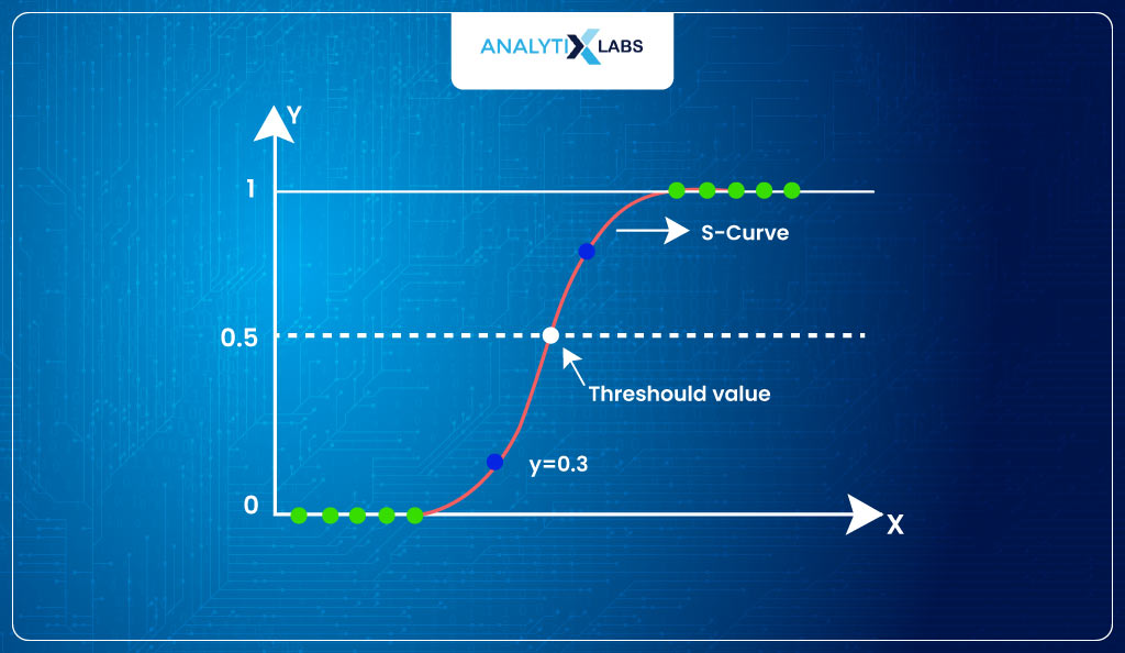
- Probability, as you might be well aware, means the likelihood of an observation belonging to class 1 based on the values of predictors. However, to get classes, you use a threshold.
- For our case, we take the threshold of 0.5 such that when the p>0.5, it returns 1; else, it returns 0.
- This way, we convert the probabilities into classes.
- However, it’s much more complicated than that, as you need to remember various misclassifications, such as false positives and negatives when finding the optimum threshold.
- Below, we use the final probabilities to convert them into classes. As you can see, there are instances where misclassification happens.

With all of this information, we hope you now have a much better understanding of how Logistic Regression works and can be interpreted.
Conclusion
Logistic Regression is a powerful algorithm that can easily solve binary classification problems. While it may be difficult to deal with when solving nonlinear problems, the algorithm has great interpretability, making it one of the most powerful tools.
It can be implemented through various tools like Python, R, SAS, and Excel.
You ought to be well prepared regarding this algorithm whenever you plan to get interviewed for a data science position, as this is one of the most fundamental algorithms popular today.
The next part of Learning Logistic Regression will include how to do logistic regression with Python [Practical learning].

![Learning Logistic Regression – Types, Algorithms, and more [Part 1 – Theory] learning logistic regression](https://www.analytixlabs.co.in/blog/wp-content/uploads/2023/09/Logistic-Regression-Theory.jpg)


